Electric Network Kernel for Support Vector Machines (Decision Theory and Optimization Algorithms)

Electric Network Kernel for

Support

Vector Machines

京都大学数理解析研究所 平井広志 (Hirai Hiroshi)

Research Institute for Mathematical Sciences, Kyoto University

東京大学大学院数理情報学専攻 室田一雄 (Kazuo Murota)

Graduate School of Information Science and Technology, University ofTokyo

ジャストシステム技術戦略室 力徳正輝 (Masaki Rikitoku)

Justsystem Corporation

R&D

Strategy Department Abstract

This paper investigates support vector machine (SVM) witha discretekernel,

named electric network kernel, defined on the vertex set ofan undirected graph.

Emphasis islaidonmathematicalanalysisof its theoretical properties withtheaid

ofelectric network theory. SVM with this kernel admits physical interpretations

in terms of resistive electric networks; in particular, the SVM decision function

corresponds to an electric potential. Preliminary computational results indicate

reasonable promise of the proposed kernel in comparison withthe Hamming and

diffusion kernels.

1

Introduction

Support vector machine (SVM) has

come

to be very popular in machine learning and

data mining communities. SVM is

a

binary classifier using

an

optimal hyperplane

learned from given training data. Through kernelfunctions, which

are a

kind of

simi-larity functions defined on the data space, the data

can

be implicitly embedded into a

high (possiblyinfinite) dimensional Hilbert space. With this kernel trick, SVM achieves

a

nonlinear classification with low computational cost.

Input data from real world problems, such

as

text data, DNA sequences and

hyper-linksinWorldWideWeb, isoften endowedwith discretestructures. Theoryand

applica-thonof “kernels

on

discrete structures”

are

pioneered by D. Haussler [5],

C. Watkins

[14]

and R. I. Kondor and J. Lafferty [8]. Haussler and Watkins independently introduced

the concept of convolution kernels. Kondor and Lafferty utilized spectral graph theory

to introduce

_diffusion

kernels, which

are

discrete kernels defined

on

vertices of graphs.

In this paper

we

propose a novel class of discrete kernels on vertices of an undirected

graph. Our approach is closely related to that of Kondor and Lafferty, but is based

on

electric network theory rather than

on

spectral graph theory. Accordingly

we

will

name

the proposed kernels electric network $ke$ nels. SVM using

an

electric network kernel

admits natural physical interpretations. The vertices with positive label and negative

potential. The resulting decision function corresponds to an electric potential, and the separating hyperplane to points with potential equal to

zero.

Emphasis is laid

on

mathematical analysis of the electric network kernel with the

aid of electric network theory.

Another

interesting special

case

is where the underlying graph is

a

tensor product ofcomplete graphs. By exploiting symmetry of this graph, we

provide

an

explicit formula for the electric network kernel, which makes it possible to

apply the electric network kernel to large-scale practical problems. In

our

preliminary

computational experimentthe electric network kernel shows fairly good performance for

some

data sets,

as

compared with the Hamming and diffusion kernels.

This paper is organized

as

follows. In Section 2, we review

SVM

and its

formu-lation as optimization problems. In

Section

3,

we

propose

our

kernel and investigate

its properties. Physical interpretations to SVM with

our

kernel

are

also explained. In

Section

4,

we

deal with the

case

of

a

tensor

product ofcomplete graphs, and show

some

computational results for

some

real world problems.

This paper is based

on

[6] but with

new

results described in Section 4.

2

Support

Vector

Machines

In this section, we review SVM and its formulation as optimization problems; see [11],

[13] for details. Let $\mathcal{X}$ be

an

input data space, e.g. $\mathrm{R}^{n}$, _{$\{0, 1\}^{n}$}, text data and DNA sequence, etc. A symmetric function $K$ : $\mathcal{X}\cross \mathcal{X}arrow \mathrm{R}$ is said to be

a

kernel

on

$\mathcal{X}$ if it

satisfies the Mercer condition:

For

any

finite subset $\mathrm{Y}$ of$\mathcal{X}$

matrix $(K(x, y)|x$,$y\in \mathrm{Y})$ is positive semidefinite. (2.1)

For

a

kernel $K$, it is well known that there exists

some

Hilbert

space

7{ with inner

product $\langle$

.,

$\cdot\rangle$ and

a

map $\phi$ : $1arrow \mathit{1}_{\mathit{4}}$ such that

$K(x, y)=\langle$

$(x),

$\phi(y)\rangle$ $(x, y\in \mathcal{X})$

.

Given

a

labeledtrainingset $(x_{1}, \eta_{1})$, $(x_{2}, \eta_{2})$,

$\ldots$ , $(x_{m}, \eta_{m})\in \mathcal{X}\cross\{\pm 1\}$,

SVM

classifier

is obtained by solving the optimization problem

$\min_{\alpha\in \mathrm{R}^{m}}$ $\frac{1}{2}\sum_{1\leq i,j\leq m}\alpha_{i}\alpha_{j}\eta_{i}\eta_{j}K(x_{i}, x_{j})-\sum_{1\leq i\leq m}\alpha_{i}$

$\mathrm{s}.\mathrm{t}$.

$\sum_{1\leq i\leq m}\eta_{i}\alpha_{i}=0,0\leq\alpha_{i}\leq C$ $(i=1, \ldots, m)$,

where $C$ is

a

penalty parameter that is

a

positive real number

or

$+$-op. If $C=+\mathrm{o}\mathrm{o}$, it

is called the hard margin $SVM$ formulation. If $C<+\mathrm{o}\mathrm{o}$, it is called the 1-norm

soft

For

our

purpose, it is convenient to consider the equivalent problem

[SVM] : $\mathrm{m}$

$u\in \mathrm{i}\mathrm{n}_{m}$ $\frac{1}{2}\sum_{1\leq i,j\leq m}u_{i}u_{j}K(x_{i}, x_{j})-\sum_{1\leq i\leq m}\eta_{i}u_{i}$

$\mathrm{s}$.t.

$1 \leq\sum_{i\leq m}u_{i}=0,$ (2.2)

$0\leq\eta_{i}u_{\iota}\leq C$ $(i=1, \ldots, m)$, (2.3)

where $u_{i}=$ ($/i\mathit{0}li$ for $i=1$, $\ldots$ ,$m$.

Let $u^{*}\in \mathrm{R}^{m}$ be

an

optimal solution of the problem [SVM] and $b^{*}\in \mathrm{R}$ be the

Lagrange multiplier ofconstraint (2.2) at $n’$. where the Lagrange function of [SVM] is

supposed to be defined

as

$L(u, \lambda, \mu, b)$ $=$ _{$\frac{1}{2}\sum_{1\leq i,j\leq m}u_{i}ujK(x_{i,j}x)-\sum_{1\leq i\leq m}\eta_{i}u_{i}$}

-$\sum_{1\leq i\leq m}\lambda_{i}\eta_{i}u_{i}-\sum_{i1\leq\sim\leq m}\mu_{i}(\eta_{i}u_{i}-C)\mathrm{i}$ $b \sum_{1\leq i\leq m}u_{i}$,

where $u\in \mathrm{R}^{m}$, $\lambda$,

$”\in \mathrm{R}_{\geq 0}^{m}$, and $b\in$ R. Then the decision function $f$ : $\mathcal{X}arrow$ $\mathrm{R}$ is given

as

$m$

$f(x)=$ $\mathrm{p}$$u_{i}^{*}K(x_{i}, x)+b^{*}$ $(x\in \mathcal{X})$. (2.4)

$i=1$

That is,

we

classify

a

given data$x$ according to thesign of$f(x)$. Adata$x_{i}$ with $\eta_{i}u_{i}^{*}>0$

is called

a

support vector. In the

case

of the 1-riorm soft margin SVM,

a

support vector

$x_{i}$ is called

a

normal support vector if $0<\eta_{i}u_{i}^{*}<C$ and a bounded support vector if $\eta_{i}u_{i}^{*}=C.$

3

Proposed Kernel and Its

Properties

Let $(V, E, r)$ be

a

resistive electric network with vertex set $V$, edge set $E$, and resistors

on

edges with the resistances represented by $r$ : $Earrow \mathrm{R}_{>0}$. We

assume

that the graph

$(V, E)$ is connected. Let $D:V\cross Varrow \mathrm{R}$ be

a

distance function

on

$V$ defined

as

$D(x, y)=$ _{resistance between} $x$ and $y$ $(X, j\in V)$

.

(3.1)

Fix

some

vertex $x_{0}\in V$

as a

root, and define a symmetric function $K$ : $V\cross Varrow \mathrm{R}$ on $V$ as

$K(x, y)=\{D(x, x_{0})+D(y, x_{0})-D(x, y)\}/2$ $(x, y\in V)$. (3.2) Seeing that $K(x_{0}, y)=0$ for all $y\in V,$

we

define

a

symmetric matrix $\hat{K}$

by

$\hat{K}=$ _{$(K(x, y)|x$},_{$y\in V\backslash \{x_{0}\})$}. (3.3)

Remark 3.1.

Given a

distance function $D$, the function $K$ defined by (3.2) is called

Let $L$ be the node admittance matrix defined as

$L(x, y)=\{$

$\mathrm{p}$

{

$(r(e))^{-1}|x$ is

an

endpoint of $e\in E$

}

if $x=y$

$-(r(xy))^{-1}$ if $x\neq y$ $(x, y\in V)$. (3.4)

If all resistances

are

equal to 1, then $L$ coincides with the Laplacian matrix of graph

$(V, E)$. Let $\hat{L}$

be asymmetric matrix defined

as

$\hat{L}=$ _{$(L(x, y)|x$},

$y\in V\mathit{3}$ $\{x_{0}\})$.

Note that $\hat{L}$

satisfies

$\hat{L}(x, y)$ $\leq$ $0$ (_$x$

a

$y$), (3.5)

$\sum_{z\in V\backslash \{x\mathrm{o}\}}\hat{L}(x, z)$

$\geq$ $0$ $(x\in V\backslash \{x_{0}\})$

.

(3.6)

Henc$\mathrm{e}$

$\hat{L}$

is a nonsingular diagonally dominant symmetric $M$-matrix. In particular, $\hat{L}$

is

positive definite. A matrix whose inverse is an $\mathrm{M}$-matrix is called an inverse M-matrix.

The following relationship between $K$ and $L$ is well known in electric network theory;

see

[4] for example.

Proposition 3.2. We have $\hat{K}^{-1}=L$

.

In particular $I\hat{\mathrm{f}}$

is

an

inverse M-matrix.

Hence, $K$ in (3.2) satisfies the Mercer condition. We shall call such $K$

an

electric

network kernel.

Remark 3.3. An electric network kernel $K$ of _{$(V, E, r)$} with root $x_{0}$ coincides with

discrete Green’s

_function

of $(V, E, r)$ taking $\{x_{0}\}$

as a

boundary condition [2].

We consider the

SVM

on

electric network $(V, E, r)$ with the kernel $K$ of (3.2). Let

$\{(x_{i}, \eta_{i})\}_{i=}1,\ldots,7m\subseteq V\cross\{\pm 1\}$ be a training data set, where

we

assume

that _{$x_{i}(i=$} $1$,

$\ldots$ ,$m$)

are

all distinct. Just as the

SVM

with a diffusion kernel, we

assume

that

$\{x_{1}, \ldots, x_{m}\}$ is

a

subset of the vertex set $V$; accordingly

we

put $V=\{x_{1}, \ldots, x_{n}\}\acute{\mathrm{w}}\mathrm{i}\mathrm{t}\mathrm{h}$

$n$ $\geq m.$

Lemma 3.4. The optimization problem [SVM] is determined independently

_of

the choice

of

a

root $x_{0}\in V$

Proof.

The objective function of [SVM] is in fact independent of$x_{0}$, since its quadratic

term can be rewritten

as

$\sum i,ju:ujK(xi, xj)$ $=$ $\sum_{\mathrm{i},\mathrm{j}}u,u_{\mathrm{j}}(D(x_{i}, x_{0})+D(xj, x_{0})-D(x_{i}, x_{j}))/2$ $=$ $\sum j^{u}j\sum iuiD(xi, x_{0})$ $-(1/2) \sum_{i,j}u_{i}u_{j}D(x_{i,j}x)$

$=$ $-(1$/2$) \sum_{i,j}u_{i}u_{j}D(x_{i}, x_{j})$,

where the last equality follows from the constraint (2.2). $\square$

Next

we

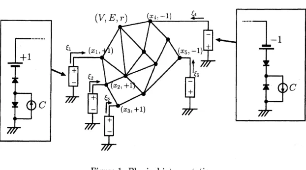
give physical interpretations to the problem [SVM] withthe aid ofnonlinear

network theory (see [7, Chapter $\mathrm{I}\mathrm{V}]$). Suppose that

we are

given

an

electric network

$(V, E, r)$ and labeled

training

data set $\{(x_{t}, \eta_{i})\}_{i=1,\ldots,m}\subseteq V\cross\{\pm 1\}$, where $x_{1}$,_$\ldots$ ,$x_{m}$

$(V, E, r)$ $x_{4}.-1)$ $\underline{arrow}\xi_{4}$

...

...

_-1

$+1$ $\xi \mathrm{r}\ulcorner$ $(x_{1}$. $)$ $(xr.-\prime 1)+$ $+$ $-\mathrm{f}_{\xi-}$ - $\xi_{-\ulcorner}$ , $x_{2}.+1$ $+$ $C$ $C$ $-+$ $\xi\ulcorner-+$ $(x_{3}.+1)$

Figure 1: Physical interpretation

For each $x_{i}$ with $1\leq i\leq m,$ connect to the earth

a

voltage

source

whose

electric potential is $\eta_{i}$ and the current flowing into $x_{i}$ is restricted to $[0, C]$

if $\eta_{i}=1$ and $[-C, 0]$ if$\eta_{i}=-1$.

By using voltage sources, current sources and diodes, this network can be realized as in

Figure 1.

Let $A=$ $(A(x, e)|x\in V$,$e\in E)$ be the incidence matrix of $(V, E)$ with

some

fixed orientation of edges and let $R=$ _diag(r(e) $|e\in E$) be the diagonal matrix whose

diagonals

are

the resistances of edges.

The electric current in this network is given

as

an

optimal solution of the problem:

[FLOW] : $\min_{(\zeta,\xi)}$

$\frac{1}{2}(^{\mathrm{T}}R(;$

$- \sum_{i=1}^{m}\eta_{i}\xi_{i}$

$\mathrm{s}.\mathrm{t}$. $A\zeta=(\begin{array}{l}\xi 0\end{array})$

$\sum_{1\leq i\leq m}\xi_{i}=0,$

$0\leq\eta_{i}\xi_{i}\leq C$ $(i=1, \ldots, m)$,

where $\langle$ represents the currents in edges and $\xi_{i}$ represents the current flowing into $x_{i}$

for $i=1$ , $\ldots$ ,$m$

.

The first and second terms of the objective function of [FLOW]

represents current potential of edges $E$ and of the voltage

sources

respectively. The

electric potential of this network is given

as

an

optimal solution of the problem: [POT] : $\mathrm{m}\mathrm{r}$ $\frac{1}{2}p^{\mathrm{T}}AR^{-1}A^{\mathrm{T}}p+C\sum_{i=1}^{m}\max\{0,1-\eta_{i}p_{i}\}$,

where $p_{i}$ represents the potential

on

vertex $x_{i}$ for $i=1$,$\ldots$ ,$n$. The first and second

terms ofthe objective function of [POT] represent voltage potentials ofedges $E$ and of

Proposition 3.5. The electric current $(\zeta^{*}, \xi^{*})$ in this network is uniquely dete rmined.

If

there exists $i\in\{1, \ldots m\}\}$ with $0<\eta_{i}\xi_{i}^{*}<C,$ then the electric potential is also

uniquely determined.

Proof.

The first assertion

follows

from the uniqueness theorem [7, Theorem 16.2]. Note

that [FLOW] and [POT]

are a dual

pair. Hence if such $\xi_{i}^{*}$ exists, from complementarity

condition, any optimal solution $p^{*}$ of [POT] must satisfy $p_{i}^{*}=\eta_{i}$. Consequently, the

potentials of other vertices

are

also uniquely determined by Ohm’s law_{$p(x)-p(y)\square =$}

$R(xy)$(;(xy) for $xy\in E$, $x$,$y\in$ $V$.

The following theorem indicates the relationship between SVM problem and this electric network.

Theorem 3.6. Let $u^{*}$ be the optimal solution

of

[SVM]. Then

$u_{i}^{*}$ coincides with the

electric current flowing into $x_{i}$

for

$i=1$, $\ldots$ ,$m$. Moreover, the decision

function

$f$

of

(2.4)

_for

[SVM] is an electric potential.

Proof.

The

problem [FLOW] is equivalent to

[FLOW] : $\min_{\xi}$ $W( \xi)-\sum_{i=1}^{m}\eta_{i}\xi_{i}$

$\mathrm{s}$.t.

$1 \leq\sum_{i\leq m}\xi_{i}=0,$

$0\leq\eta_{i}\xi_{i}\leq C$ $(i=1, \ldots, m)$,

where $W:\mathrm{R}^{m}arrow \mathrm{R}$is defined

as

$W( \xi)=\min_{\zeta}\{\frac{1}{2}\zeta^{\mathrm{T}}R\zeta|A\zeta=(\begin{array}{l}\xi 0\end{array})$$\}1$

By the

Lagrange

multiplier method,

we

can

easily show that

$W( \xi)=\frac{1}{2}1\leq$

V

$m\xi_{i}\xi_{j}K(x_{i}, x_{:})$

.

This implies that the problem [FLOW] coincideswith [SVM]. Next

we

show the latter

part. From the fact that [FLOW] and [POT] are a dual pair, it can be shown that

the decision function $f$ : $Varrow \mathrm{R}$ defined by (2.4) satisfies the optimality condition of

[POT]. $\square$

From Proposition 3.5 and Theorem 3.6,

we

see

that the electric potential coincides

with the decision function of [SVM], provided that the optimal solution of [SVM] has

a

normal support vector. Furthermore, the

Lagrange

multiplier $b^{*}$ corresponds to the

electric potential ofthe root vertex $x_{0}$, if the potential is normalized in such

a

way that

the earth has

zero

electric potential.

Next

we

consider the

case

of the hard-margin

SVM.

The following proposition

Proposition 3.7. For the electric network kernel If,

an

optimal solution u

_of

the unconstrained optimization problem

[SVM’] : $\min$ _{$\frac{1}{2}\sum_{1\leq l,j\leq m}u_{i}u,\cdot K(x_{i}, x_{j})-\sum_{1\leq i\leq m}\eta_{i}u_{i}$} $u6\mathrm{R}^{m}$

$\mathrm{s}.\mathrm{t}$.

$\sum_{1\leq i\leq m}u_{i}=0$

is also optimal to [SVM] with $C=+ao$.

Proof.

Suppose that $/i$ $=+1$ for $1\leq i\leq k$ and $\eta_{i}=-1$ for $k+1\leq i\leq m.$ By

a

variant

of Lemma 3.4,

we

may take $x_{m}$

as

the root. Then problem [SVM’] is equivalent to $u \mathrm{m}_{m-1}^{\mathrm{i}\mathrm{n}}1\sum_{1\leq i,j\leq m-1}u_{i}u_{j}K(x_{i}, x_{j})-\sum_{1\leq i\leq k}2u_{i}$,

where

we

substitute $u_{m}=- \sum_{1\leq i\leq m-1}u_{i}$ in [SVM’]. Let $\overline{K}=(K(x_{i},x_{j})|1\leq i,j\leq$

$m-1)$

.

Hence the optimal solution $u^{*}\in \mathrm{R}^{m}$ is given by

$u_{i}^{*}$ $=$

$2 \sum_{1\leq j\leq k}(\overline{K}^{-\tilde{1}})_{ij}$ $(1\leq i\leq m-1)$, $u_{m}^{*}$ $=$ -2

$\sum_{1\leq j\leq k}$$\sum_{1\leq h\leq m-1}(\overline{K})_{hj}1$

.

Since $\overline{K}$

is an inverse $M$-matrix by Proposition 3.2,

we

have

$u_{i}^{*}\geq 0$ $(1 \leq i\leq k)$, $u_{i}^{*}\leq 0$ $(k+1\leq i\leq m)$.

Hence $u^{*}$ satisfies the inequality constraint of [SVM] and is optimal. $\square$

Hence, in the case of the hard-margin SVM, the following correspondence holds.

SVM

electric network

positive label data +1 voltage

sources

negative label data -1 voltage

sources

optimal solution of [SVM] electric current from voltage

sources

decision function electric potential

The following corollaries immediately follow from these physical interpretation, where

we

assume

the hard-margin

SVM.

Corollary

3.8.

Let$u^{*}\in \mathrm{R}^{m}$ be the optimalsolution

of

[SVM]. Then,

for

_{$i\in\{1, \ldots, m\}$},

$x_{i}$ is a support vector, &.$e.$, $\mathit{7}\mathit{1}:>0$

if

and only

if

there exists

a

path

from

$x_{i}$ to

some

_$Xj$

with $\eta_{i}\neq\eta_{j}$ such that it contains no other labeled training vertex (data).

Suppose thatthereexists

some

trainingdata$x$ such that the deletion of$x$from $(V, E)$

makes two

or more

connected components, i.e., $x$ is an articulation point of $(V, E)$

.

Let

$U_{1}$,

$\ldots$ ,$U_{k}$ be the vertex sets of the connected components after the deletion of $x$

.

Let

$(U_{1}\cup\{x\}, E_{1})$, _$\ldots$, $(U_{k}\cup\{x\}, E_{k})$ be subgraphs of $(V, E)$. Restricting training data set

to each subgraph,

we

obtain

SVM

problems $[\mathrm{S}\mathrm{V}\mathrm{M}_{1}]$,

$\ldots$ ,

Corollary 3.9. Under the above assumption, the optimal solution

_of

[SVM]

can

be

represented

as

the

sum

_of

optimal solutions

_of

$[\mathrm{S}\mathrm{V}\mathrm{M}_{1}]$,

$\ldots$ ,

$[\mathrm{S}\mathrm{V}\mathrm{M}_{\mathrm{k}}]$. Consequently,

for

each$i\in\{1, \ldots, k\}$, the restriction to $U_{i}\cup\{x\}$

of

the decision

function

of

the hard-margin

[SVM] coincides with the decision

_{function of}

$[\mathrm{S}\mathrm{V}\mathrm{M}_{i}]$.

Remark 3.10. SVM with

an

electric network kernel falls in the scope of discrete

convex

analysis [9], which is a theory of

convex

functions with additional combinatorial

struc-tures. Specifically, the objective function of [SVM] with

an

electric network kernel is an

$M$

-convex

function

in continuous variables, and the optimization problem [SVM] is

an

$\mathrm{M}$

-convex

function minimization problem.

Remark 3.11. Smola and Kondor [12] consider various kernels constructed from the

Laplacian matrix $L$ of

an

undirected graph _{$(V, E)$}. In particular, they introduced the

kernel

$K=(I+\sigma L)^{-1}$,

where $\sigma$ is

a

positive parameter. In

our

view, this kernel corresponds to the electric

network kernelof

a

modifiedgraph $(V\cup\{x_{0}\}, E\cup\{yx_{0}|y\in V\})$with

a

newly introduced

root vertex $x_{0}$.

The computation of elements of$D$

or

$K$ through numerical inversion of $\hat{L}$

is highly

expensive because the size of $\hat{L}$

is usually very large. In Section 4, we consider an

N-tensor product of$k$-complete graphs that admits efficient computation of the elements

of $K$.

4

SVM

on

Tensor Product

of Complete Graphs

4.1

Explicit

formula for

the

resistance

In this section,

we

consider the

case

where $(V, E)$ is

an

$N$-tensor product offc-complete

graphs defined

as

$V$ $=$ $\{0, 1, 2, \ldots, k-1\}^{N}$.

$E$ $=$ $\{xy|x, y\in V, d_{\mathrm{H}}(x, y)=1\}$,

where $d_{\mathrm{H}}$ : $V\mathrm{x}Varrow \mathrm{R}$is the Hamming distance defined

as

$d_{\mathrm{H}}(x, y)=\{i\in\{1, \ldots, /\mathrm{V}\}|x^{i}\neq y^{i}\}$,

where $x^{i}$ denotes the $i$th component of$x\in V,$

In the

case

of $k=2,$ this graph coincides with

an

$N$-dimensional hypercube. We

regard $(V, E)$

as an

electric network where all resistances of edges

are

equal to 1. Hence

the node

admittance

matrix of $(V, E)$ coincides with

the

Laplacian matrix.

By symmetry of this graph, the resistance $D$ between two vertex pair is given

as

a function in the Hamming distance of the pair

as

follows. The proof is presented in

Theorem

4.1. The resistance D : $\mathrm{T}^{\gamma}\cross Varrow \mathrm{R}$

of

an

_$N$-tensor product

of

k-complete

graphs $(\mathrm{T}^{\gamma},$E) is given by

$D(x, y)=$

$\{$

$\frac{1}{2^{N-2}}\sum_{s=1,3,5}^{d},\ldots\sum_{u=0}^{N-d}$ $(\begin{array}{l}ds\end{array})(\begin{array}{l}N-du\end{array})$_{$\frac{1}{2(s+u)}$} if $k=2,$

$s=1,3,5,\ldots$ $100 \sum_{u=0}^{Nd}(_{S}^{d})(^{d-s}t)(_{u}^{N-d})$

$\cross\frac{2^{2-s}k^{-N+s+t+u}}{k(s+t+u)}(\frac{1}{2}-\frac{1}{k})^{t}(1-\frac{1}{k})^{u}$ if $k\geq 3$,

(4.1)

where $d=d_{\mathrm{H}}(x, y)$.

The theorem implies, in particular, that each element of kernel $K$

can

be computed

with $O(N^{4})$ arithmetic operations. This makes it possible to apply the electric network

kernel to large-scale practical problems on this class of graphs.

Remark 4.2. The computationalefficiency of the formula (4.1) relies essentially

on

the

fact that the number ofdistinct eigenvalues ofthe Laplacian matrixof$(V, E)$ is bounded

by $O(N)$;

see Subsection

4.3. In a

more

general

case

where the _{graph is}

an

N-tensor

product of complete graphs of different sizes, the number of distinct eigenvalues may

possibly be exponential in $N$

.

Our approach in Subsection 4.3 hints at

a

difficulty of

obtaining

a

computationally efficient formula for this class of graphs.

4.2

Experimental results

Here, we describe preliminary experiments with

our

electric network kernels

on

tensor

products of complete graphs. In order to estimate the performance,

we

compare the

electric network kernel with the Hamming kernel and the diffusion kernel [8] using

benchmark data having binary attributes. By the Hamming kernel

we mean

the kernel

defined

as

$K(x, y)=N-d_{\mathrm{H}}(x, y)$ $(x, y\in\{0,1\}^{N})$

.

The

diffusion kernel

and the electric network kernel

are

implemented to

LIBSVM

pack-age

[1], which is

one

of the

common

SVM package

programs.

For benchmark data

sets,

we use

Hepatitis, Votes, LED2-3, and Breast Cancer taken from UCI Machine

LearningRepository [10] (Table 4.1). Forthe first three datasets,

we

regard theseinput

spaces

as

hypercubes, i.e., $k=2$ _in (4.1). In Hepatitis data set,

we use

12 binary

at-tributes ofall 20 attributes. LED2-3 data set is made through the data generating tool

in [10] by adding 10% noise. For Breast Cancer data set,

we

regard its input space

as

9-tensor product of 10-complete graphs, i.e., $N=9$ and $k=10$ in (4.1).

Table4.2 shows theexperimentalresults with Hammingkernel (HK), diffusion kernel

(DK), and electric network kernel (ENK) for these datasets, whereAce

means

theratio

of correct

answers

averaged

over 40

random 5-fold

cross

validations and

SVs

is the

Table 4.1: Data sets

Data set Size Positive Negative Attribute

Hepatitis 155 32 123 12

Votes 435 168 267 16

LED2-3 1914 937 977 7

Breast Cancer 699 251

458

9

Table

4.2:

Experimental results

$\mathrm{H}\mathrm{K}$ DK ENK

Data set

SVs

Ace

(C)

SVs

Ace

$(C, \beta)$

SVs

Acc

(C)

Hepatitis 60 79.125 (64) 60 79.775 (256, 3.5) 106

77.725

(256)

Votes 36

95.975

(4.0) 53 .025 (512, 3.0) 274 84.450 (128)

$\mathrm{L}\mathrm{E}\mathrm{D}2-3$

386

89.550 (2.0) 392 89.700 (0.2, 3.0) 388 89.800 (70)

$\underline{\mathrm{B}\mathrm{r}\mathrm{e}\mathrm{a}\mathrm{s}\mathrm{t}}$Cancer152

$-9\underline{7.271(0.02)242}$

97.000(2,0.3) 463 81.713 (200)

HK $=$ Hamming kernel, DK $=$ diffusion kernel, ENK $=$ electric network kernel.

the soft margin parameter $C$ and the diffusion

coefficient

4

achieving the best

cross

validated

error

rate.

For Hepatitis and LED2-3 data sets, three kernels show almost equivalent

perfor-mance.

For Votes and Breast Cancer data set, However,

our

ENK shows somewhat

poor performance than others. In Hepatitis, Votes, and Breast Cancer, ENK has

larger

SVs

than other kernels. This phenomenon

can

be explained by Corollary

3.8 as

follows. Since these three data sets

are

well separated than LED2-3, the soft margin

SVM with ENK is close to the hard margin SVM. Hence it is expected from Corollary

3.8 that these

SVM

with ENK have many $\mathrm{S}\mathrm{V}\mathrm{s}$

.

The above results indicate that

our

electric network kernel works well

as

an SVM

kernel. It is fair to

say,

however, that

more

extensive experiments against various kinds of data sets

are

required before its performance

can

be confirmed with

more

precision

and confidence. Comprehensive computational study is left as a future research topic.

4.3

Proof of

Theorem 4.1

First,

we

consider the spectra of

a

$k$-complete graph. Let $L$ be the Laplacian matrix of

a

$\mathrm{f}\mathrm{c}$-complete graph with vertex set $[k]=\{0,1, \ldots, k-1\}$, i.e.,

$L(x, y)=\{$ $k-1$ if $x=y$ $(x, y\in[k])$. -1 otherwise

Lemma 4.3. L has the eigenvalues 0 with multiplicity 1 and k with multiplicity k–1.

The eigenvector

_for

0 is given by

$p_{0}=$ $(\begin{array}{l}11\vdots 1\end{array})$ (4.2)

and the eigenvectors

_for

$k-1$ are given by

$p_{1}=\{$ 1 $\backslash$ $-1$ 0 . $\cdot$ . / , $p_{2}=(\begin{array}{l}1\mathrm{l}-20\vdots\end{array})$ : $p_{3}=($ 1 $\backslash$ $1$ 1 -3 0 . $\cdot$ . $\int$

, $\ldots’.p_{k-1}=$ $(\begin{array}{ll} 1 1 \vdots 1-k +1\end{array})$ (4.3)

Let $\Lambda$ and

$g$ be diagonal matrices with diagonalelements given by

$\Lambda(x)=\{$ 0if $x=0$

$k$ otherwise

$(x\in[k])$, (4.4)

$g(x)=\{$ $1/k$ if $x=0$

$1/x(x+1)$ otherwise $(x\in[k])$, (4.5)

and $P$ and $Q$ be matrices defined as

$P(x, y)=p_{y}^{x}$, $Q(x, y)=g(x)P(y, x)$ $(x, y\in[k])$, (4.6) where $p_{y}^{x}$

means

the $x$-component of the eigenvector $p_{y}$

.

By the orthogonality of$p_{y}$’S,

we

have

$\sum_{z\in[k]}P(x, z)Q(z, y)=\delta(x, y)$ $(x, y\in[k])$, (4.7)

where $\delta$ is the Kronecker’s delta. Then _$L$

can

be diagonalized

as

$L(x, y)= \sum_{z\in[k]}\Lambda(z)P(x, z)Q(z, y)$ $(x, y\in[k])$. (4.8)

Second,

we

derive the diagonalization of the Laplacian matrix $L_{N}$ of

an

\^A-tensor

product of $k$-complete graphs. Note that $L_{N}$

can

be represented

as

From (4.7) and (4.8), $L_{N}$

can

be diagonalized

as

$L_{N}(x, y)$ $=$ $\sum N\sum\Lambda(z^{i})P(x^{i}, z^{i})Q(z^{i}, y^{i})$

$\prod N$ $\sum P(x^{j}, z^{j})Q(z^{j}, y^{j})$

$i=1z^{i}\in[k]$ $r=$l,i-ji$z^{j}\in[k]$

$= \sum_{z\in[k]^{N}}(\sum_{i=1}^{N}\Lambda(z^{i}))\prod_{j=1}^{N}P(x^{j}, z^{j})Q(z^{j}, y^{j})$

$= \sum_{z\in[k]^{N}}\Lambda_{N}(z)P_{N}(x, z)Q_{N}(z, y)$

$(x, y\in[k]^{N})$,

where $\Lambda_{N}$, $P_{N}$ and $Q_{N}$

are

defined

as

$\Lambda_{N}(x)=\sum_{i=1}^{N}\Lambda(x^{i})$, $P_{N}(x, y)= \prod_{j=1}^{N}P(x^{j}, y^{j})$, $Q_{N}(x, y)= \prod_{j=1}^{N}Q(x^{\mathrm{j}}, y^{j})$ $(x, y\in[k]^{N})$.

(4.9)

Note that $Q_{N}$ is the inverse of$P_{N}$.

Finally,

we

drive the formula for the resistance. We take$0=$ (0,0, $\ldots$,0)

as

the root.

Let $\hat{L}_{N},\hat{P}_{N}$ and $\hat{Q}_{N}$ be the restrictions of _{$L_{N}$}, $P_{N}$ and $Q_{N}$ to $[k]^{N}\backslash \{0\}$ respectively.

Then

we

have

$\hat{L}_{N}(x, y)$

$= \sum_{z\in[k]^{N}\backslash \{0\}}\Lambda_{N}(z)\hat{P}_{N}(x, z)\hat{Q}_{N}(z, y)$

$(x, y\in[k]^{N}\backslash \{0\})$,

$(\hat{L}_{N})^{-1}(x, y)$

$= \sum_{z\in[k]^{N}\backslash \{0\}}(1/\Lambda_{N}(z))(\hat{Q}_{N})^{-1}(x, z)(\hat{P}_{N})^{-1}(z, y)$

$(x, y\in[k]^{N}\backslash \{0\})$

.

From the fact that $P_{N}$ is the inverse of $Q_{N}$ and definitions of $Pn$_, $Q_{N}$, $P$ and $Q$, it is

easy to verify that

$(\hat{P}_{N})^{-1}(x, y)$ $=$ $Q_{N}(x, y)-Q_{N}(x, 0)Q_{N}(0, y)/Q_{N}(0,0)$

$=g_{N}(x)(P_{N}(y, x)-1)$,

$(\hat{Q}_{N})^{-1}(x, y)$ $=$ $P_{N}(x, y)$$)-P_{N}(x, 0)P_{N}(0, y)/P_{N}(0,0)$ $=$ $P_{N}(x, y)-1,$

where $g_{N}(y)= \prod i_{=1}g(y^{i})$

.

Hence

we

have

$D$(x,$0$)

$=K(x, x)= \hat{L}_{N}^{-1}(x, x)=\sum_{z\in[k]^{N}\backslash \{0\}}\frac{g_{N}(z)}{\Lambda_{N}(z)}(P_{N}(x, z)-1)^{2}$

.

(4.10)

$(x, 0)$

$–[-k]^{N}$

Let $s=\# A,$ $t=\# B$ and $u=\# C$ with $s+t+u$ $\neq 0$ Then we have

$\sum_{z\in 6_{A,B,C}^{\tau}}\frac{g_{N}(z)}{\Lambda_{N}(z)}(P_{N}(x, z)-1)^{2}$

$= \sum_{z\in S_{A,B,C}}\frac{g_{N}(z)}{k(s+t+u)}(\prod_{i=1}^{d}P(1, z^{i})\prod_{i=d+1}^{N}P(0, z^{i})-1)^{2}$

$= \frac{\{(-1)^{s}-1\}^{2}}{k(s+t+u)}\sum_{z\in S_{A_{1}B,C}}\prod_{i=1}^{N}g(z^{i})$

$= \frac{\{(-1)^{s}-1\}^{2}}{k^{\wedge}(s+t+u)}\sum_{z\in S_{A_{1}B,C}}g(1)^{s}g(0)^{N-s-t-u}\prod_{i\in B}g(z^{i})\prod_{j\in C}g(z^{j})$

$= \frac{\{(-1)^{s}-1\}^{2}}{k(s+t+u)}2^{-s}k^{-N+s+t+u}$

$\cross.\prod_{-\prime \mathrm{D}}(\frac{1}{6}[perp]\ldots+\frac{1}{k(k+1)}).\prod_{-\wedge\cap}(\frac{1}{2}+\frac{1}{6}+\cdots+\frac{1}{k(k+1)})$

$= \sum_{z\in S_{A,B,C}}\frac{g_{N}(z)}{k(s+t+u)}(\prod_{i=1}^{u}P(1, z^{i})\prod_{i=d+1}^{\mathit{1}\prime}P(0, z^{i})-1$

$= \frac{\{(-1)^{s}-1\}^{2}}{k(s+t+u)}\sum_{z\in S_{A_{1}B,C}}\prod_{i=1}^{\mathrm{J}\prime}g(z^{i})$

$= \frac{\{(-1)^{s}-1\}^{2}}{k^{\wedge}(s+t+u)}\sum_{z\in S_{A_{1}B,C}}g(1)^{s}g(0)^{N-s-t-u}\prod_{i\in B}g(z^{i})\prod_{j\in C}g(z^{j})$

$= \frac{\{(-1)^{s}-1\}^{2}}{k(s+t+u)}2^{-s}k^{-N+s+t+u}$

$\cross.\prod_{p*\subset}(\frac{1}{6}[perp]\ldots+\frac{1}{k(k+1)}).\prod_{-\prime\cap}(\frac{1}{2}+\frac{1}{6}+\cdots+\frac{1}{k(k+1)})$ $\cross i\in B11(\overline{6}\overline{k(k+1)})[perp]\ldots+j$

J\inJC

$(\overline{2}\overline{6}\overline{k(k+}++\cdots+$ $= \frac{\{(-1)^{s}-1\}^{2}}{k(s+t+u)}2^{-s}k^{-N+8+t+u}(\frac{1}{2}-\frac{1}{k})^{t}(1-\frac{1}{k})^{u}$

In the

case

of$k>3.$ we _have

$D(x, 0)$

$= \sum_{C\subseteq}\sum_{zA,B\subseteq\{\begin{array}{l}1\prime d\{\}\end{array}\},A\cap B=\emptyset\in S_{A,B,C}}\frac{g_{N}(z)}{\Lambda_{N}(z)}(P_{N}(x, z)-1)^{2}$

$= \sum_{s=1,3}^{d},\ldots\sum_{t=0}^{d-s}\sum_{u=0}^{N-d}$$(\begin{array}{l}ds\end{array})(\begin{array}{l}d-st\end{array})(\begin{array}{l}N-du\end{array})$ $\frac{2^{2-s}k^{-N+s+t+u}}{k(s+t+u)}(\frac{1}{2}-\frac{1}{k})^{t}(1-\frac{1}{k})^{u}$

In the

case

of$k=2$_, $B$ must be empty, and hence

we

have

$D(x, 0)$ $=$

$c^{A\subseteq\{1,..d\}} \subseteq \mathrm{t}d+\mathrm{i},.,N\sum_{\prime}..’$$\sum_{z\in S_{A,9,C},\}}\frac{g_{N}(z)}{\Lambda_{N}(z)}(P_{N}(x, z)-1)^{2}$

$=$ $\sum_{s=1,3}^{dN},\ldots$$\sum_{u=0}^{-d}$ $(\begin{array}{l}ds\end{array})(\begin{array}{l}N-du\end{array})$$\frac{2^{2-s}2^{-N+s+u}}{2(s+u)}(1-\frac{1}{2})^{u}$

$=$ $\frac{1}{2^{N-2}}\sum_{\mathrm{s}=1,3}^{d},\ldots$$\sum_{u=0}^{N-d}\frac{1}{2(s+u)}$$(\begin{array}{l}ds\end{array})(\begin{array}{l}N-du\end{array})$

.

Acknowledgement

$\mathrm{S}$

The authors thank Satoru Iwata and Shiro Matuura for helpful suggestions. This work

is

an

outcome of

a

joint project between University ofTokyo and Justsystem Co. This

$= \sum_{s=1,3}^{a},\ldots\sum_{t=0}^{a-s}\sum_{u=0}^{N-d}$$(\begin{array}{l}ds\end{array})(\begin{array}{l}dt\end{array})(\begin{array}{l}Nu\end{array})$ $\frac{2^{2-s}k^{-N+s+t+u}}{k(s+t+u)}(\frac{1}{2}-\frac{1}{k})^{t}(1-\frac{1}{k})^{u}$

In the

case

of$k=2$_, $B$ must be empty, and hence

we

have

$D(x, 0)$ $=$

$c^{A\subseteq\{1} \sum_{\subseteq\{d+}$

,$\mathrm{i}\cdot,\cdot.’..,Nd\},$,

$\}\sum_{z\in S_{A,,9,C}}\frac{g_{N}(z)}{\Lambda_{N}(z)}(P_{N}(x, z)-1)^{2}$

$=$ $\sum_{s=1,3}^{d},\ldots\sum_{u=0}^{N-d}$ $(\begin{array}{l}ds\end{array})(\begin{array}{l}Nu\end{array})$ $\frac{2^{2-s}2^{-N+s+u}}{2(s+u)}(1-\frac{1}{2})^{u}$

$=$ $\frac{1}{2^{N-2}}\sum_{s=1,3}^{d},\ldots\sum_{u=0}^{N-d}\frac{1}{2(s+u)}$$(\begin{array}{l}ds\end{array})(\begin{array}{l}Nu\end{array})$

Acknowledgement

$\mathrm{S}$

The authors thank Satoru Iwata and Shiro Matuura for helpful suggestions. This work

work is also supported by the 21st Century COE Program on Information Science and

Technology Strategic Core, and

a Grant-in-Aid

for Scientific Research from the Ministry

ofEducation, Culture, Sports,

Science

and Technology of Japan.

References

[1] C. C. Chang and C. J. Lin: LIBSVM a library for support vector machines, 2001. Software available at http:$//\mathrm{w}\mathrm{w}\mathrm{w}$.csie. ntu.edu.$\mathrm{t}\mathrm{w}/\sim \mathrm{c}\mathrm{j}\mathrm{l}\mathrm{i}\mathrm{n}/\mathrm{l}\mathrm{i}\mathrm{b}\mathrm{s}\mathrm{v}\mathrm{m}$

[2] F. Chung and S.-T. Yau: Discrete Green’s functions, Journal

_of

Combinatorical

Theory Series A 91 (2000),

no.

1-2, 191-214.

[3] D. M. Cvetkovic’, M. Doob and H. Sachs: Spectra

_of

Graphs, 3rd. ed., Johann

Am-brosius Barth Verlag, Heidelberg-Leipzig, 1995.

[4] M. Fiedler:

Some

characterizations ofsymmetric inverse $M$-matrices, Linear Algebra

and Its Applications 275/276 (1998),

179-187.

[5] D. Haussler: Convolution kernels

on

discrete structures, Technical report

UCSC-CRL-99-10, Department of Computer Science, University of California at Santa

Cruz, 1999.

[6] H. Hirai, K. Murota and M. Rikitoku: SVM Kernel by Electric Network, METR

2004-41, University of Tokyo, August, 2004.

[7] M. Iri: Network Flow, Transportation and Scheduling, Academic Press, New York,

1969.

[8] R. I. Kondor and

J.

Lafferty:

Diffusion

kernels

on

graphs and other discrete

struc-tures, in: C.

Sammut

and A. Hoffmann, eds., Proceedings

_of

the 19th International

Conference

on

Machine Learning, Morgan Kaufmann, 2002,

315-322.

[9] K. Murota: Discrete

Convex

Analysis, SIAM, Philadelphia, PA,

2003.

[10] P. M. Murphy and D. W. Aha:

UCI

Repository

_of

machine learning databases,

http:$//\mathrm{w}\mathrm{w}\mathrm{w}.$ics.uci.edu/-mlearn/MLRepository.html, Irvine,

CA:

Universityof

California, Department ofInformation and Computer Science,

1994.

[11] B. Sch\"olkopf and A. J. Smola: Learning with Kernels, MIT Press, 2002.

[12] A. J. Smolaand R. Kondor: Kernels and regularization

on

graphs, in: B. Scholkopf

and M. Warmuth, eds., Proceedings

_of

the Annual

_Conference

on

Computational

Learning Theory

and

Kernel Workshop, Lecture

Notes

in Computer

Science

2777, Springer,

2003.

[13] V. Vapnik: Statistical Leaning Theory, Wiley,

1998.

[14] C. Watkins: Dynamic alignment kernels, in: A. J. Smola, B. Schoklopf, P. Barlett,

and D. Schuurmans, eds.,

Advances

in Large-Margin Classifiers, MIT Press 2000,