EXISTENCE AND STABILITY OF A TRAVELING WAVE SOLUTION ON A 3-COMPONENT REACTION-DIFFUSION MODEL IN COMBUSTION (Nonlinear evolution equations and mathematical modeling)

EXISTENCE AND STABILITY OF A TRAVELING WAVE SOLUTION ON A

3-COMPONENT

REACTION-DIFFUSION

MODEL IN COMBUSTION

KOTA IKEDA ANDMASAYASU MIMURA

1. INTRODUCTION

It is shown in [8] that thin solid, for an example, paper, cellulose dialysis bags and polyethylene sheets, buming against oxidizing wind develops finger-like patterns or fingering patterns. The oxidizing $gtL\backslash$ is

supplied in a uniformlaminar flow, opposite to the directions of the front propagation and they control the flowvelocityof

oxygen,

denotedby $V$

.

When$V$isdecreased belowacritical value, thesmoothfront develops

a structurewhich marks the onsetofinstability. As $V$ isdecrea.sed further, the peaks

are

separated by

cusp-like minima and a fingering pattern is formed. In addition, thin solid is stretched out straight onto the bottom plate and they also control the adjustable vertical gap, denoted by aparameter $h$, between top and

bottom plates. We remark here that fingering patterns occur for small $h$, which implies that such patterns

appearin the absence ofnatural convection. Similar phenomena have been also observed in

a

micro-gravity experiment in space (see [5]).

To investigate these phenomena, a reaction-diffusion model (RD) $w:\backslash propcx\backslash ed$ in [2]. We carried out

numerical simulations, reproducing similar results to the experiment described above. If the effect of the flow (denoted by $\lambda$ in (RD)) is strong, aflame front is smooth. Decreasing$\lambda$ raises the destabilization of the smooth flame front. Eventually, fingering pattern

occurs

in small $\lambda>0$

.

Our model (RD) is represented as follows:

$(RD)$ $\{\begin{array}{l}\frac{\partial u}{\partial t}=Le\Delta u+\lambda’\frac{\partial u}{\partial x}+\gamma k(u)vw-au,\frac{\partial v}{\partial t}=-k(u)vtlJ,\frac{\partial_{tl\prime}}{\partial t}=\Delta_{8l\prime}+\lambda\frac{\partial_{ll)}}{\partial x}-k(u)vw,\end{array}$ $(x,y)\in(-\infty, \infty)\cross\zeta l,$$t>0$,

where the constants $Le$, called Lewis number, $\gamma$ and $a$

are

positive constants,

$\lambda$ and $\lambda’$

are

nonnegative

constants, $\zeta l\subset \mathbb{R}^{\iota}$ is a bounded domain, and $\Delta=\partial^{2}’\partial x^{2}+\sum_{i=1}^{l}\partial^{2}’\partial r/^{2}|$ is Laplacian

as

usual. The

nonlinear term $k$ is defined by

$k(u)=\{\begin{array}{ll}A \exp(-B/(tl-\theta)), u>\theta,0, 0\leq u\leq\theta\end{array}$

for some constants $A,$$B>0$ and $\theta\geq 0$. This function $k$ and $\theta$ are called Arrhenius kinetics and ignition temperature incombustion. Note that we considered a general setting for the nonlinear function $k$ in [2] and

[3].

We suppose that

$\lim u(x,y, t)=0$, $\lim_{xarrow\infty}\tau n(x,y,t)=tl_{r}’>0$, $\lim_{xarrow-\infty}w(x,y,t)=\tau n_{l}\geq 0$ $|x|arrow\infty$

for any $y\in\zeta l$ and$t>0$, where $\tau n_{r}$ and $\tau n_{\iota}$

are

$C0IL\backslash tant\backslash$ and $tlJ_{r}>tl$)$1$

.

We also$f^{\backslash },tlppo_{\iota}\backslash \backslash e$ that $u$ and$w$ satisfy $\frac{\partial u}{\partial\nu}(x,y,t)=0$, $\frac{\partial_{ll)}}{\partial\nu}(x,y,t)=0$

for $x\in(-\infty, \infty),$ $y\in\partial\zeta]$ and $t>0$, where $\nu$ is the unit exterior normal vector

on

$\partial\ddagger l$

.

We suppose that initial fiunctions satisfy

and

(1.1) $tl_{0}’(+\infty, y)=?l)_{\mathcal{T}}$, $?l10(-\infty, y)=?I_{\text{ノ}l}’$

.

In numericalsimulations, asmooth flame front

is

observed in (RD) if$\lambda$ is sufficiently large, which implies that (RD) $h_{tk}s$ a stable traveling

wave

solution independent of y-variable. Our first aim in this

paper

is to

construct a

stable traveling

wave

solution in the

case

that $\lambda$ islarge. The second

aim

will be described after

the

statement

of

Theorem 3.

Now

we

describe main results and how to prove the existence and stability of

a

traveling

wave solution

of (RD). We formally take the limit of$\lambdaarrow\infty$ in (RD) so that $\partial\tau v’\partial x=0$ holds. Then, from the boundary

condition of $w$,

we

obtain $\tau v\equiv w_{r}$ and (RD) is reduced to

(1.2) $\{\begin{array}{l}\frac{\partial u}{\partial t}=Le\Delta u+\lambda’\frac{\partial u}{\partial x_{\text{ノ}}}+\gamma k(\uparrow 4)vtl_{r}^{1-au},,(x, y)\in(-\infty, \infty)\cross\zeta l, t>0\frac{\partial v}{\partial t}=-k(u)v\tau v_{r}\end{array}$

with the boundary condition

$\lim_{|x|arrow\infty}u(x,y, t)=0$, $y\in\Omega,$$t>0$,

$\frac{\partial u}{\partial\nu}(x,y, t)=0$, _{$x\in(-\infty, \infty),$}$y\in\partial\Omega,$$t>0$

.

Hence a solution of (RD) approaches that of (1.2). Theorem 1. Let $(u^{\lambda\lambda\lambda}v, \tau r))$ be a solution

of

$(RD)$ with an _initial

function

$(u_{0}^{\lambda}, v_{0}^{\lambda}, uJ_{0}^{\lambda})$ depending

on

$\lambda$ and $(u,v)$ be a solution

_of

(1.2) ivith an initial

_function

$(u_{0}, v_{0})$

.

Suppose that $(u_{0}^{\lambda}, v_{0}^{\lambda})$ and $(u_{0}, v_{0})$ belong

to $D(L_{u}^{\alpha})\cross C^{\kappa}((-\infty, \infty)\cross\zeta l)$ and satisfy

(1.3) $\Vert u_{0}^{\lambda}-u_{0}\Vert_{\alpha}arrow 0$, $||v_{0}^{\lambda}-v_{0}\Vert_{L^{\infty}((-\infty,\infty)x\Omega)}arrow 0$

as

$\lambdaarrow\infty$

.

Here $L_{u}^{\alpha}$ is a

fractional

power

of

_{$L_{u}\equiv-Le\Delta-\lambda’\partial’\partial x+a$} with the domain

$D(L_{u}^{\alpha})$ endowed

by $\Vert\cdot\Vert_{\alpha}\equiv\Vert\cdot\Vert_{Lp((-\infty,\infty)x\Omega)}+\Vert L_{u}^{\alpha}\cdot\Vert_{L^{p}((-\infty,\infty)x\Omega)}$

for

1 $2<\alpha<1$ and $n+1<p<\infty$ (see [6]), and

$C^{\kappa}((-oo\infty)\cross\Omega)$ i$ a Holder space with the exponent _$0<\kappa<1$

.

In addition,

assume

$w_{0}^{\lambda}-\eta\in D(L_{z}^{\alpha})$,

where a monotonically increasing

_function

$\eta\in C^{2}(-\infty, \infty)$ satisfy

$\eta(x)=\{\begin{array}{l}7l\prime_{r}, x\geq 1,w_{1}, x\leq 0,\end{array}$

and $L_{z}^{\alpha}$ is a

fractional

power

of

$L_{z}\equiv-\Delta-\lambda\partial’\partial x$. Then,

for

any _$\delta,T>0$ and$R\in$ $(-$oo $\infty)$,

$\sup_{0<t<T}(\Vert u^{\lambda}(t)-u(t)\Vert_{\alpha}+\Vert v^{\lambda}(t)-v(t)\Vert_{L^{\infty}((-\infty,\infty)x\Omega)})arrow 0$,

(1.4)

$\sup_{\delta<t<T}||\tau v^{\lambda}(t)-?lJ_{r}\Vert_{L^{\infty}((R,\infty)x\Omega)}arrow 0$

as $\lambdaarrow\infty$

.

From this result, a traveling

wave

solution of (RD) may approach that of (1.2). In order to achieve

our

goal,

we

introduce a

new

parameter $\epsilon>0$ and construct a solution of

(1.5) $\{\begin{array}{l}-\epsilon cu’=\epsilon^{2}u’’+\epsilon\lambda’u’+\gamma k(u)vtl)r-au,-\alpha\prime’=-k(u)vtlfr\end{array}$

with boundary conditions

(1.6) $u(\pm\infty)=0$, $v(+\infty)=v_{r}$,

where $c$ is called

wave

speed of a traveling

wave

solution. We derived (1.5) from (1.2) by putting $Learrow\epsilon$,

$\gammaarrow\gamma\epsilon$, and $aarrow a\epsilon$

.

Although this problem is easierthan (1.8) and (1.9) below, it is stilldifficult to verify

the existence of a traveling wave solution without any technical $li_{\wedge}\backslash Stlmptionn$ for parameters. Ifwe

use

the

smal parameter $\epsilon$,

we can

apply perturbation theory toour problem and construct atraveling wave solution.

By this method

we

also

see

how the traveling

wave

solution obtained in the following theorem behaves $1k’i$

Theorem 2 ([3]). $S\uparrow\nu$ppose that th

$e\tau e\uparrow.s\underline{v}$ such that

for

any$\underline{\uparrow)}<?1$, it holds that

$\int_{0}^{u_{1}(\underline{v})_{(\gamma k(u)\underline{v}\uparrow l)_{f}}}-au)du=0$,

where $u_{1}(v)$ denotes the maximum

of

the three

zeroes

of

$\gamma k(u)v\tau v_{r}-au$

.

Then, there

are

positive

constants

$\overline{v}$ and _{$\lambda’(v_{r})$} such that

if

$\underline{v}<v_{r}<\overline{v},$ $0\leq\lambda’<\lambda’(v_{r})$, and $\epsilon>0$ is sufficiently small, the system (1.5) with

(1.6) has

a

solution, denoted by $(u, v, c)$

.

In addition, the associated eigenvalue problem

(1.7) $\{\begin{array}{l}\epsilon\mu\phi=\epsilon^{2}\phi’’+\epsilon(c+\lambda’)\phi’+\gamma k’(u)v\tau n_{r}\phi+\gamma k(u)u)r\psi-a\phi,\mu\psi=r\psi’-k’(u)v\tau v_{r}\phi-k(u)\psi\end{array}$

has a unique solution $(\phi, \psi, ’ 4)=(\uparrow\iota’, \uparrow)’,$$0)$ in $H_{\kappa}^{2}(\mathbb{R})\cross H_{\kappa}^{1}(\mathbb{R})\cross\Lambda_{\delta}$

for

small_{$\kappa>0,$ $u$)}$hereH_{\kappa}^{1}(\mathbb{R})$ and $H_{\kappa}^{2}(\mathbb{R})$

are weighted Sobolev spaces, and $\Lambda_{\delta}$ is a closed subset in $\mathbb{C}$

for

small $\delta>0$

defined

later. The two small

pammeters $\kappa$ and

5 are

supposed to be independent

of

$\epsilon$

.

$F\}_{4}rthemore$ the algebmic multiplicity

of

$\mu=0$ is 1 in (1.7).

A traveling

wave

solution is (Iinearly) stable ifthe eigenvalue problemdoes not have

an

eigenvalue $\mu\in\Lambda_{\delta}$

except for $\mu=0$, and the algebraic multiplicity of $\mu=0$ is 1. Note that $(u’, v’)$ is a solution of (1.7) for $\mu=0$

.

Since $k(O)=0$ and $k’(O)=0$, the $e_{\grave{\backslash }\grave{2}\grave{\cdot}!}\backslash entia1$spectra come to the imaginary axis if we consider the above problem in a usual Lebesgue space or continuous function‘s space (see Section 5 in [1]). In order to avoid the essential spectra of (1.10), it is necessary to introduce weighted functional spaces. We define

a

functional space $L_{\kappa}^{2}(\mathbb{R})$ by

$L_{\kappa}^{2}( \mathbb{R})=\{\varphi\in L_{loc}^{1}(\mathbb{R})|\Vert\varphi\Vert_{L_{\kappa}^{2}}\equiv(\int_{-\infty}^{\infty}|\varphi(z)|^{2}e^{2\kappa z}dz)^{1\prime 2}<\infty\}$

.

Sobolev spaces $H_{\kappa}^{1}(\mathbb{R})$ and $H_{\kappa}^{2}(\mathbb{R})$ with the weight fumction $e^{\kappa z}$

are

defined $1i_{\wedge}^{s}lL_{\kappa}^{2}(\mathbb{R})$ analogously. If

we

&$\backslash$

sume

that the eigenfumction belongs to the weighted space, the eigenvalue problem (1.10) does not have essential spectra in $\mu\in\Lambda_{\delta}$ for

a

small $\delta>0$ Hence it is sufficient to consider only spectra with a finite

multiplicity (namely, eigenvalues), where $\Lambda_{\delta}$ is defined by

$\Lambda_{\delta}=\{\mu\in \mathbb{C}|{\rm Re}\mu\geq-\delta\}$

and ${\rm Re}\mu$ is the real part of 4. Although we only consider the linear stability in this paper, it may imply the

usual stability.

From Theorems 1 and 2, we

can

easily obtain a stable traveling wave

so

lution in (RD)

as a

perturbed solution of (1.5) and (1.6). However, we cannot obtain a traveling wave solution in (RD) byonly Theorems 1 and 2 because Theorem 1 determines the behavior of solutions in (RD) and (1.2) in local time. We have to give a rigorous proofin order to establish the existence of a traveling wave solution in (RD).

We follow the argument above and use thesmall parameter $\epsilon$

.

Our problem is given by

(1.8) $\{\begin{array}{l}-\epsilon cu’=\epsilon^{2}u’’+\epsilon\lambda’u’+\gamma k(u)v\uparrow l)-au,-cv’=-k(u)vtl),-\alpha JJ’=w’’+\lambda w’-k(u)vw,\end{array}$

and boundary conditions

(1.9) $u(\pm\infty)=0$, $v(+\infty)=v_{r}>0$, $\tau rj$($+$oo) _$=Tl)r$ ’

where the spatial coordinate $z$ is given by

$z=x-ct$

.

Theorem 3. Under the same conditions as in Theorem 2,

_if

$\lambda$ is sufficiently large, there is a traveling

wave

solution, denoted by $(u, v, \tau lj, c)$

of

(1.8) and (1.9). In addition, the associated eigenvalue problem

has a unique solution $(\phi, \psi, \eta, ]I)=(u’, t’, 1l_{\text{ノ^{}\prime}}^{l}, 0)$ in $H_{\kappa}^{2}(\mathbb{R})\cross H_{\kappa}^{1}(\mathbb{R})\cross C_{\kappa}(\mathbb{R})\cross\Lambda_{\delta}$, where $C_{\kappa}(\mathbb{R})$ is

defined

by

$C_{\kappa}(\mathbb{R})=\{\eta\in C(\mathbb{R})|_{-\infty<z<\infty}L\backslash ;\iota 1p|\eta(z)|e^{\kappa z}<\infty\}$.

Furthermore the

algebmic

multiplicity

_of

$\mu=0$ is 1.

So far we have been investigating a traveling wave solution which represents flame uniformly burning against oxidizing wind. By numerical calculation

we

observe another type ofsolutions in (RD), “reflection of traveling

wave

solutions” (see Figure I, [4]). Our second aim in this

paper

is to $coi_{L}sider$ the

reflection

phenomena

in

(RD).

Actiially, reflection

cannot be

seen

in the $ci_{k}se$ that $\lambda i_{\iota}s$ large.

In

the above

we

only

consider a traveling wave solution under the condition that $\lambda$ is sufficiently large, which cannot be applied to reflection phenomena. Then we constriict a soliition of (1.8) with $\lambda$ fixed again.

$\sim\cdot\cdot r\cdots\cdot\cdot**\cdot\cdot$

$t=100$ $t=400$

FIGURE 1. Reflection of a traveling

wave

soliition. In this figure, three lines (one solid line and two dotted lines) represent the functions $T,$ $P$, and $W$, respectively. This numerical

calculation

was

done in a finite interval. The traveling

wave

solution initially goes to right (the left figure). After it hits the boundary, a different traveling

wave

solution arises (the right figiire).

Theorem 4. Fix$\lambda$

.

Under the

same

$c,ondihons$ as

in $Theore_{d}m2$_, there is a _travelingwave _solution

_of

_(1.8)

and (1.9).

We also consider other traveling

wave

solution in (RD) in the opposite direction of the previous traveling

wave

solution andstudy

(1.11) $\{\begin{array}{l}\epsilon(,u’=\epsilon^{2}u’’+\epsilon\lambda’u’+\gamma k(u)vw-au,rv’=-k(u)v\uparrow l),Ctl’\prime=tlJ’’+\lambda w’-k(u)vw,\end{array}$

and boundary conditions

(1.12) $u(\pm\infty)=0$, $v(-\infty)=v_{r}$, $\tau v(+\infty)=rn_{r}$

.

Theorem 5. Fix$\lambda inde,pendent$

of

$\epsilon$

.

Under the same conditions as in Theorem 2, there is a traveling

wave

solution

_of

(1.8) and (1.9).

Here weremark arelated $res\iota ilt$on the existence ofa travelingwave solution of (1.5). $Thi_{f}$; is the work of

Roques [7]. In this work, the author proved the exititence ofatraveling

wave

solutionin a combustionmodel with

an

ignition temperatiire (i.e. $\theta>0$ in the definition of _$k(u)$) without using any singiilar perturbation theory. This result implies that (1.5) $hi_{k}s$ only two traveling

wave

solutions with different

wave

speeds.

However, this work does not contain the

case

where $k(u)$ is not of ignition type, namely, _{$k(u)>0$for $u>0$}

.

In addition, the stability of _{those traveling wave solutions is unclear although it} may be believed that a traveling

wave

solution with a faster wave speed is stable and a traveling

wave

solution with aslower

wave

speed is unstable in general. On the other hand, we prove the existence of a traveling wave solution even in

the

case

of$\theta=0$. Furthermore, we also show the stability of that traveling wave solution by using a singular

perturbation theory.

This paper is organized $ti\backslash \backslash$ follows. In what follows

we

only give

an.

outline of the proof for Theorems 4 and 5. In the proof we apply singular perturbation theory. We formally $co$nstruct solutions, called outer and inner solutions.

2. CONSTRUCTION

OF A TRAVELING WAVE SOLUTION IN $($

1.8

$)$ AND $($

1.11

$)$

In this section

we

construct

a

formal

solution

of

(1.8)

and

(1.11).

We

$f;etzarrow-z$

_{and rewrite}

$(1\cdot.8)$

into

(2.1) $\{\begin{array}{l}\epsilon c,u’=\epsilon^{2}u’’-\epsilon\lambda’u’+\gamma k(u)vtlj-au,cv’=-k(u)vw,(^{\backslash }?l^{\prime=w-\lambda_{tlj}’-k(u)v?l1},\end{array}$

andboundary conditions

(2.2) $u(\pm\infty)=0$, $v(-\infty)=v_{r}$, $tlj$($-$oo) $=t1J_{f}$

.

We first construct outer and inner solutions of this problem. We divide $(-\infty, \infty)$ into three parts

$I_{1}=(-\infty, 0)$, $I_{2}=(0, \tau)$, $I_{3}=(\tau, \infty)$

.

The width of the second interval is a parameter denoted by $\tau$, which is determined later.

From

the second

and third equations of (2.1), we have

$tl)”-((\backslash +\lambda)w’=k(u)vw=-cv’$

.

Byintegrating $(-\infty, z)$, it holds that

$tl)’-(c+\lambda)(?lJ-tl)r)=-c(v-v_{r})$

.

We treat this equation instead of the third equation of (2.1). Finally,

we

consider

on

each intervals

(2.3) $\{\begin{array}{ll}\epsilon^{2}u^{(1)’’}-\epsilon(c+\lambda’)u^{(1)’}+\gamma k(u^{(1)})v^{(1)}w^{\langle 1)}-au^{(1)}=0, z\in I_{1},cv^{(1)’}+k(u^{(1)})v^{(1)_{tl)}(1)}=0, z\in I_{1},1l)\langle 1)’-(r, +\lambda)(\tau v^{\langle 1)}-?l\prime_{r})=-c(v^{(1)}-v_{r}), z\in I_{1},\end{array}$

(2.4) $\{\begin{array}{ll}\epsilon^{2}u^{(2)’’}-\epsilon(c+\lambda’)u^{\langle 2)’}+\gamma k(u^{\langle 2)})v^{(2)_{Tl)}\langle 2)}-au^{(2)}=0, z\in I_{2},r,v^{\langle 2)’}+k(u^{(2)})v^{(2)}\uparrow l\text{ノ} (2) =0, z\in I_{2},t11(2)’-(c+\lambda)(\tau^{(2)}ll-\tau\downarrow\prime_{r})=-c(v^{(2)}-v_{r}), z\in I_{2},\end{array}$

and

(2.5) $\{\begin{array}{ll}\epsilon^{2}u^{(3)’’}-\epsilon(c+\lambda’)u^{(3)’}+\gamma k(u^{(3)})v^{(3)_{kI)}(3)}-au^{(3)}=0, z\in I_{3},(\gamma J\langle a)’+k(u^{\langle 3)})v^{\langle 3)_{tl)}\langle 3)}=0, z\in I_{3},\tau\ell^{\langle 3)’(3)}J-(c+\lambda)(1l’-?Ijr)=-c(v^{(3)}-v_{f}), z\in I_{3}.\end{array}$

Also,

we

construct aformal solution of (1.11) by dividing $(-\infty, \infty)$ into three parts

$I_{1}=(-\infty, 0)$, $I_{2}=(0, \tau)$, $I_{3}=(\tau, \infty)$

.

Since our traveling

wave

solution is expected to be bounded, the function $\tau n$ must

converge

to a constant,

proceeds, $1l_{l}$ must be nonnegative and less than $\tau/;_{\tau}$. By the same argument as above, we replace the third

equation of(1.11) into a first-order differential equation and consider on each intervals

(2.6) $\{\begin{array}{ll}\epsilon^{2}u^{(1)’’}+\epsilon(\lambda’-c)u^{(1)’}+\gamma k(u^{(1)})v^{(1)}w^{(1)}-au^{(1)}=0, z\in I_{1},(w^{(1)’}+k(u^{(1)})v^{(1)}w^{(1)}=0, z\in I_{1},\end{array}$

(2.7) $\{\begin{array}{ll}\epsilon^{2}u^{(2)’’}+\epsilon(\lambda’-c)u^{\langle 2)’}+\gamma k(u^{(2)})v^{(2)}w^{(2)}-au^{(2)}=0, z\in I_{2},r,v^{(2)’}+k(u^{(2)})v^{(2)_{1lj}(2)}=0, z\in I_{2},\end{array}$ $u^{\langle 1)’}’+(\lambda-c)(w^{(1)}-u)\iota)=-c(v^{(1)}-v_{r})$_{, $z\in I_{1}$,}

$\tau^{(2)’(2)}lj+(\lambda-r,)(\uparrow 1\mathfrak{i}-\tau vl)=-c(v^{(2)}-v_{r})$_,

$z\in I_{2}$,

and

(2.8) $\{\begin{array}{ll}\epsilon^{2}u^{\langle 3)’’}-\epsilon(\lambda’-r)u^{(3)’}+\gamma k(u^{(3)})v^{(3)}w^{(3)}-au^{\langle 3)}=0, z\in I_{3},(,v^{(3)}’-k(u^{(3)})v^{(3)}w^{(3)}=0, z\in I_{3},t^{(3)’(3)}lj+(\lambda-c)(\uparrow l)-w_{l})=-c(v^{(3)}-v_{r}), z\in I_{3}.\end{array}$

The nonnegative constant $w_{l}$ will be determined later.

2.1. The lowest order approximation of (2.1). We first construct outersolutions. By putting $\epsilon=0$in

(2.3), we formally get

$\{\begin{array}{ll}\gamma k(U_{0}^{(1)})V_{0}^{\langle 1)}W_{0}^{\langle 1)}-aU_{0}^{(1)}=0, z\in(-\infty, 0),(,V_{0}^{(1)’}+K(U_{0}^{(1)})V_{0}^{(1)}W_{0}^{(1)}=0, z\in(-\infty, 0),W_{0}^{(1)’}-(c+\lambda)(W_{0}^{(1)}-\tau v_{r})=-c(V_{0}^{(1)}-v_{r}), z\in(-\infty, 0),V_{0}^{(1)}(-\infty)=v_{r}, W_{0}^{(1)}(-\infty)=ujr.\end{array}$

From the first and second equations it holds that $U_{0}^{(1)}(z)=0$ and $V_{0}^{(1)}(z)=v_{r}$

.

Then $W_{0}^{(1)}(z)$ is given by

$W_{0}^{(1)}(z)=w_{r}-Ae^{(c+\lambda)z}$

for a constant $A$ determined later.

Next, by putting $\epsilon=0$ in (2.4),

we

formally get

$\{\begin{array}{ll}\gamma k(U_{0}^{(2)})V_{0}^{(2)}W_{0}^{(2)}-aU_{0}^{(2)}=0, z\in(0, \tau),cV_{0}^{(2)’}+k(U_{0}^{(2)})V_{0}^{(2)}W_{0}^{(2)}=0, z\in(0, \tau),W_{0}^{(2)’}-(c+\lambda)(W_{0}^{(2)}-w_{r})=-c(V_{0}^{(2)}-v_{r}), z\in(0, \tau),V_{0}^{(2)}(0)=V_{0}^{(1)}(0), W_{0}^{(2)}(0)=W_{0}^{(1)}(0).\end{array}$

Let $p=h_{+}(q)$ be

a

unique _{positive solution of$\gamma k(p)q-aq=0$}

.

_{Then the first equation}

_can

_{be solved with}

respect to $U_{0}^{(2)}$ such

rus

_{$U_{0}^{(2)}(z)=h_{+}(V_{0}^{(2)}(z)W_{0}^{(2)}(z))$}

.

Substitutingit into the second equation,

we

have

$\{\begin{array}{ll}cV_{0}^{(2)’}=-k(h_{+}(V_{0}^{(2)}W_{0}^{(2)}))V_{0}^{\langle 2)}W_{0}^{(2)}, z\in(O, \tau),W_{0}^{(2)’}-(c+\lambda)(W_{0}^{(2)}-w_{r})=-c(V_{0}^{\langle 2)}-v_{r}), z\in(0, \tau),V_{0}^{(2)}(0)=v_{r}, W_{0}^{(2)}(0)=tl\prime_{r}-A. \end{array}$

It is easy to see the

existence

of the solution of this problem by standard theory for ordinary differential equations.

By putting $\epsilon=0$ in (2.5), we formally get

$\{\begin{array}{ll}\gamma k(U_{0}^{(.})V_{0}^{(.i)}W_{0}^{(:}-aU_{0}^{(.)}=0, z\in(\tau, \infty),cV_{0}^{(3)’}+k(U_{0}^{(3)})V_{0}^{(3)}W_{0}^{(3)}=0, z\in(\tau, \infty),W_{0}^{\langle 3)}’-(c+\lambda)(W^{(3)}0-u)r)=-c(V_{0}^{(3)}-v_{f}), z\in(\tau, \infty),V_{0}^{(3)}(\tau)=V_{0}^{(2)}(\tau), |W_{0}^{(3)}(+\infty)|<\cdot\infty.\end{array}$

Traveling wave solutions

are

supposed to

be

bounded. We supposed that $W_{0}^{(3)}$ satisfies the boundary

condition at $\infty$

.

Then, by the similar argument above,

we

have $U_{0}^{(3)}(z)\equiv 0,$ $V_{0}^{(3)}(z)\equiv V_{0}^{(2)}(\tau)$, and $W_{0}^{(3)}(z)\equiv\tau v_{r}+c(V_{0}^{(2)}(\tau)-v_{r})/(c+\lambda)$.

Next

we

consider the inner solution at $z=0,$$\tau$. At $z=0$,

we

introduce the stretched variable $\xi=z’\epsilon$

.

Rewrite (2.1) by using $\xi$ and putting $\epsilon=0$

.

Then we formally get

$\{\begin{array}{l}\ddot{\phi}_{0}-(c+\lambda’)\phi_{0}+\gamma k(\phi_{0})v_{r}(w_{r}-A)-a\phi_{0}=0, \xi\in(-\infty, \infty),\phi_{0}(-\infty)=0, \phi_{0}(\infty)=U_{0}^{(2)}(0)(=h_{+}(v_{r}(TI)_{T^{-A)))}},\end{array}$

where $($ ‘”

denotes the differentiation with respect to $\xi$

.

There is

$\overline{A}$

such that for

any

given $0<A<\overline{A}$,

this

problem ha.$s$ a solution $\Phi_{1}(\xi)$ with a

wave

speed uniquely determined, denoted by ($,$ $=(;^{*}(A)$

.

The constant

$\overline{A}$ is given such

as

the

wave

speed c’$(A)$ corresponds to $0$ for $A=\overline{A}$

.

Note that _$c^{*}(A)$ is continuous with

respect to $A$ and decreii.ses monotonically.

Before we consider the inner solution at $z=\tau$, we first define $\alpha((;)$ and $\Phi_{1}(\xi)$

.

Let $\alpha(c)$ be a positive

constantsuch as the problem

$\{\begin{array}{l}\ddot{\phi}-(r, +\lambda’)\dot{\phi}+\alpha(c)\gamma k(\phi)-a\phi=0, \xi\in(-\infty, \infty),\phi_{0}(-\infty)=h_{+}(\alpha(c)), \phi_{0}(\infty)=0\end{array}$

$ha.\cdot$; a solution _{$\Phi_{1}(\zeta)$} for each $0<c,$ $<\overline{(\backslash }$

.

We denote the maximum

wave

speed by $\overline{r}$, i.e., $\overline{c}$is such apositive constant $lki$ this problem does not have

a

traveling

wave

solution for$c>\overline{(;}$

.

Now

we

introduce the stretched variable$\xi=(z-\tau)\epsilon$ andobtain

an

innersolution at _$z=\tau$

.

We formally obtain

$\{\begin{array}{ll}\ddot{\phi}_{0}-(c+\lambda’)\dot{\phi}_{0}+\gamma k(\phi_{0})V_{0}^{(2)}(\tau)W_{0}^{(2)}(\tau)-a\phi_{0}=0, \xi\in(-\infty, \infty),\phi_{0}(-\infty)=U_{0}^{(2)}(\tau)(=h_{+}(V_{0}^{(2)}(\tau)W_{0}^{(2)}(\tau))),\phi_{0}(\infty)=0.\end{array}$

If $V_{0}^{\langle 2)}(\tau)W_{0}^{(2)}(\tau)$ _Is equal to $\alpha(c)$, this problem ha.$s$ a solution $\phi_{0}(\xi)=\Phi_{2}(\zeta)$

.

We have defined allouterand inner solutions. Recall that thewavespeed (,must be$c^{*}(A)$ for the existence

of$\Phi_{1}(\xi)$

.

Then, substituting _$c=c^{*}(A)$ into the outer and inner solutions, we formally express our traveling

wave solution $(u, v, ?l))a_{\backslash }s$

$(u, v,tl;)\sim\{\begin{array}{ll}(\Phi_{1}(\frac{z}{\epsilon}), v_{r}, W_{0}^{(1)}(z)), z\in I_{1},(U_{0}^{(2)}(z)+(\Phi_{1}(\frac{z}{\epsilon})-U_{0}^{(2)}(0))+(\Phi_{2}(\frac{z-\tau}{\epsilon})-U_{0}^{(2)}(\tau)), V_{0}^{(2)}(z), W_{0}^{(2)}(z)), z\in I_{2},(\Phi_{2}(\frac{z}{\epsilon}), V_{0}^{(2)}(\tau), ?l)_{\Gamma}+\frac{t^{*}(A)(V_{0}^{(2)}(\tau)-v_{r})}{(^{*}(A)+\lambda}), z\in I_{3}.\end{array}$

Unfortunately, the function $rv$ is not continuous at $z=\tau$ in general. In addition, we do not

see

that there

does exist the function $\Phi_{2}(\xi)$, that is, $V_{0}^{(2)}(\tau)W_{0}^{(2)}(\tau)$correspond to $\alpha(c)$

.

Toestablish these two conditions,

we must choose

an

appropriate pair $(A, \tau)$, which is given in the next lemma.

Lemma 1. There is a pair$(A^{*}, \tau^{*})$ such that it

satisfies

Proof.

To prove this lemma, we evaluate the behavior of the solution of a differential equation

(2.10) $\{$

$c^{*}(A)v’=-k(h+(v\uparrow v))\tau)?I1$, _{$z>0$ ,} $w’-(r^{*}(A)+\lambda)(\tau v-w_{r})=-c^{*}(A)(v-v_{r})$_{, $z>0$,} $v(0)=v_{r}$, $w(0)=u)r^{-A}$

in the v-iv phase space. In particular it is important to study the A-dependency ofthe solution.

We introduce

some

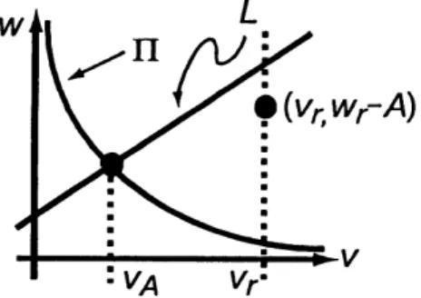
notations here (see Figure 2). We define

a

line $L$ and ahyperbolic

curve

$\Pi$ by

$L=\{(v,w)|(r^{*}(A)+\lambda)(w-w_{r})=c^{*}(A)(v-v_{r})\}$, $\Pi=\{(v, w)|vw=\alpha((,*(A))\}$,

respectively. The line $L$ isthrough $(v_{r}, tlJ_{r})$, while$\Pi$ is below $(v_{r}, ?I_{r}’)$ becauseof$\alpha(c^{*}(A))<v_{r}?lJ_{r}$

.

The slope

of$L$ is positive so that $L$ intersects $\Pi$ at a unique point in _$v>0,$$\uparrow l$) $>0$, denoted by $(vA, wwA)$. It is obvious

that $vA<v_{r}$ and $?vA<t1i_{r}$

.

Let $\Gamma$ be asegment defined by

$\Gamma=\{(v, \tau v)\in L\cup\Pi|v_{A}<v<v_{r}\}$

.

In what follows, we show that thesolution of (2.10) is through the intersection $(v_{A,A}w)$ for some $A$

.

We note that$v’$ is strictlynegative for positive $v$ and$w$, the initial value of(2.10) is below $(v_{r’ r}tl))$ in the

phasespace. Due to the continuity and monotonicity of$c^{*}(A)$ with respect to $A,$ $(v_{r}u’-A)$ is beneath $L$

and above $\Pi$

.

Hence the flow of (2.10) must hit $\Gamma$ at some

$z$ for $0<A<\overline{A}$, denoted by $z^{*}(A)$

.

It iseasy to

see

that $z^{*}(A)$ is uniquely determined. Since the solution of (2.10) continuously dependson theinitial value

and parameters, $z^{*}(A)$ is continuous with respect to$A$

.

We finally prove that there is $A$ such that _{$(v(z^{*}(A)), ?l,’(z^{*}(A)))=(v_{A}, tI^{1A})$} for

some

$A$

.

If $A$ is close

to $0$, the initial value is

near

_{$(v_{r}, tl_{r})\in L$}

.

Then _$v$ decreases more than

$\tau v$ for small

$z>0$

so

that $(v(z^{*}(A)), w(z^{*}(A)))$ _{must be} on $L$ at _$z^{*}(A)$

.

On the other hand, _$c^{*}(A)$ tends to $0$ as $Aarrow\overline{A}$, and then

the slope of $L$ also tends to $0$

.

Since

$?1_{\overline{A}}=\tau rjr$ is larger than $\uparrow\downarrow$)$r^{-\overline{A}}’(v(z^{*}(A)), \tau v(z^{*}(A)))$ must be on $\Pi$ at $z^{*}(A)$

.

From these facts and the continuity of $c^{*}(A)$ and $z^{*}(A)$ with respect to $A$, we can conclude that

there is $A^{*}$ such that _{$(v(z^{*}(A^{*})), tI1(z^{*}(A^{*})))$}matches _{$(v\cdot\tau ij)$} by the intermediate value theorem. We

put

$\tau^{*}=z^{*}(A^{*})$

.

$\square$

FIGURE 2. The line $L$ and the hyperbolic curve $\Pi$ in the $v-\tau r$) plane. There is a unique

intersection of$L$ and $\Pi$, which corresponds to _{$(v_{A,R}11))$}

.

2.2. The lowest order approximation of (1.11). In thissubsection we obtain outer and inner solutions for (1.11) by taking the limit of$\epsilonarrow 0$

.

When we construct the solutions,

we

need the relationship between $\lambda$ and thewave speed

$c$

.

In the next lemma, we prove that $\lambda$ must be larger than $c$

.

Lemma 2.

_If

there is a bounded solution

_of

(1.11) and (1.12), the

wave

speed$c$ is less than $\lambda$

.

Pmof.

By the second equation of (1.11) and $uarrow 0$

as

$zarrow\infty,$ $v(+\infty)$ exists and $v(+\infty)<v_{r}$

.

From the

third equation of (1.11),

we

have

$(\lambda-c)(t1J_{r}-w_{t})=-c(v_{r}-v(+\infty))<0$

.

We first construct outer solutions by the similar argument in the previous section. By putting $\epsilon=0$ in

(2.6), we have

$U_{0}^{(1)}(z)=0$, $V_{0}^{(1)}(z)=v_{r}$, $W_{0}^{(1)}(z)=w_{l}$

.

By putting$\epsilon=0$ in (2.7), we formally get $U_{0}^{(2)}=h_{+}(V_{0}^{(2)}W_{0}^{(2)})$, and $(V_{0}^{(2)}, W_{0}^{(2)})$ is a solution of

$\{\begin{array}{ll}cV_{0}^{(2)’}=-k(h_{+}(V_{0}^{\langle 2)}W_{0}^{(2)}))V_{0}^{(2)}W_{0}^{(2)}, z\in(O,\tau),W_{0}^{(2)’}+(\lambda-r)(W_{0}^{(2)}-w_{1})=c(v_{r}-V_{0}^{(2)}), z\in(0,\tau),V_{0}^{(2)}(0)=v_{r}, W_{0}^{(2)}(0)=u)_{\iota}.\end{array}$

Finally, by putting $\epsilon=0$ in (2.8), we have $U_{0}^{(3)}(z)=0$, $V_{0}^{(3)}(z)=V_{0}^{(2)}(\tau)$,

$W_{0}^{\langle 3)}(z)=(u)_{\iota}- \frac{c}{\lambda-c}’(V_{0}^{(2)}(\tau)-v_{r}))(1-e^{-(\lambda-c)(z-\tau)})-W_{0}^{(2)}(\tau)e^{-\langle\lambda-c)(z-\tau)}$

.

Note that $W_{0}^{(2)}(\tau)=W_{0}^{(3)}(\tau)$ holds. From the boundary condition for the function $\tau\iota$) at

$\infty,$ $W_{0}^{(3)}(+\infty)$ $=?lj\iota-c(V_{0}^{(2)}(\tau)-v_{r})’$₍$\lambda-(^{\backslash },)$ must be equal to $tI$)

$r$. However it does not hold true in general. We will find

an

appropriate value $7lj\iota$ later.

Next we consider the inner solutions at $z=0$ and $z=\tau$

.

At $z=0$, we introduce the stretched variable

$\xi=z’\epsilon$

.

Rewrite (1.11) by using $\xi$ and putting$\epsilon=0$

.

Then we formally get

(2.11) $\{\begin{array}{ll}\ddot{\phi}_{0}+(\lambda’-c)\dot{\phi}_{0}+\gamma k(\phi_{0})v_{r^{tI)}}\iota-a\phi_{0}=0, \xi\in(-\infty, \infty),\phi_{0}(-\infty)=0, \phi_{0}(\infty)=U_{0}^{(2)}(0)(=h_{+}(v_{r}?lj_{\iota))}.\end{array}$

This problem $h$_}$k^{\backslash }i$ a solution $\Phi_{1}(\xi)$ with a wave speed $c=c^{*}(rv_{1})$ uniquely determined for each $\tau v_{l}>8l\rangle_{*}$, where $w_{*}$ is given such $t\mathfrak{B}$ c’$(w.)=0$

.

Since

our

interest is in traveling

wave

solutions with

a

positive

wave

speed,

we

naturally

assume

this condition. In addition we should consider the upper boumd for $?l$)$lbeca\iota i_{f^{\backslash },e}$

$c^{*}(w\iota)$ must be smaller than $\lambda$ from Lemma 2. Hence we suppose that $tl’\iota$ satisfies $w_{*}<w\iota<\tau n^{*}$, where $?l)^{*}$ are defined as follows. The constant

$TI$)‘ is supposed to be $tl$)$r$ in the case of $\lambda>c’$$(\tau n_{r})$, while in the

case

of $\lambda\leq c^{*}(2l)r)$, it is defined such $tk^{\backslash }tc^{*}(?l)^{*})=\lambda$

.

The wave speed $c^{*}(\tau n_{l})$ is continuous and incre&set

monotonically so that $\tau n_{*},$$\tau v^{*}$ are uniquely determined.

At $z=\tau$, we introduce the stretched variable $\xi=(z-\tau)\epsilon$ and formally get

$\{\begin{array}{ll}\ddot{\phi}_{0}+(\lambda’-c)\dot{\phi}_{0}+\gamma k(\phi_{0})V_{0}^{(2)}(\tau)W_{0}^{(2)}(\tau)-a\phi_{0}=0, \xi\in(-\infty, \infty),\phi_{0}(-\infty)=U_{0}^{\langle 2)}(\tau)(=h_{+}(V_{0}^{\langle 2)}(\tau)W_{0}^{\langle 2)}(\tau))) \phi_{0}(\infty)=0.\end{array}$

If $V_{0}^{(2)}(\tau)W_{0}^{(2)}(\tau)$ is equal to $\alpha(c^{*}(kl)\iota))$ for $tl_{l}$, this problem has a solution denoted by $\Phi_{2}(\xi)$, where $\alpha wi_{k^{\backslash }}$;

defined in the previous section.

We have already defined all outer and inner solutions of (1.11). Recall that the

wave

speed $c$ must be $c^{*}(\tau v\iota)$ for the existence of $\Phi_{1}(\xi)$

.

Then, substituting $(, =c^{*}(?l)\iota)$ into the outer and inner solutions,

we

formally express

our

traveling wave soliition $(u,v, w)\iota\iota\backslash$;

$(u,v,w)\sim\{\begin{array}{ll}(\Phi_{1}(\frac{z}{\epsilon}), v_{r}, \tau v_{1}), z\in I_{1},(U_{0}^{(2)}(z)+(\Phi_{1}(\frac{z}{\epsilon})-U_{0}^{(2)}(0))+(\Phi_{2}(\frac{z-\tau}{\epsilon})-U_{0}^{\langle 2)}(\tau)), V_{0}^{(2)}(z), W_{0}^{(2)}(z)), z\in I_{2},(\Phi_{2}(\frac{z}{\epsilon}), V_{0}^{\langle 2)}(\tau), W_{0}^{(3)}(z)), z\inI_{3}.\end{array}$

The function $?l$) does not satisfy the boundary condition at $z=+\infty$ in general $tk9$ described previously. In

addition, we do not

see

that there does exist the function $\Phi_{2}(\xi)$, that is, $V_{0}^{(2)}(\tau)W_{0}^{(2)}(\tau)$ corresponds to

$\alpha(c^{*}(klil))$

.

To establish these two conditions, we must choose

an

appropriate pair $(w_{l}, \tau)$, which is given in

Lemma 3. There is apair $(Tl^{\tau^{*}},, \mathcal{T}^{*})$ such that it

satisfie

$s$

(2.12) $\{$

$? 1)\iota-\frac{c_{\vee}^{*}(7lil)}{\lambda-c^{*},(\tau v_{l})}(V_{0}^{(2)}(\tau)-?)r)=tl;_{r}$,

$V_{0}^{(2)}(\tau)W_{0}^{\langle 2)}(\tau)=\alpha(c^{*}(\uparrow l1\iota))$

.

Proof.

We

first introduce several notations. Let $(v,\tau v)$ be

a

solution of

(2.13) $\{\begin{array}{ll}c^{*}(w_{t})v’=-k(h_{+}(vtl’))v\uparrow l1, z>0,?l)’+(\lambda-r^{*}(?If_{\iota))(?v-kl1l)=-c^{*}(?l)}\iota)(v-v_{r}), z>0,v(0)=v_{r}, w(0)=w_{l}.\end{array}$

Define two lines $L_{1},$ $L_{2}$ and a hyperbolic

curve

$\Pi$ by

$L_{1}=\{(v, w)|(\lambda-c^{*}(w_{l}))(tl’-\tau r_{l})=-c^{*}(\tau v_{l})(v-v_{r})\}$, $L_{2}= \{(v,\uparrow l))|v=v_{r}-\frac{\lambda-c^{*}(\tau r_{\text{ノ^{}\prime}l})}{r_{d}^{*}(w\iota)} ($ _で砺 $-?ll\iota)\}$,

$\Pi=\{(v, \uparrow lj)|v\uparrow lJ=\alpha(r^{*}(\uparrow lj_{l}))\}$

.

Since the slope of $L_{1}$ is negative, $L_{1}$ intersects $\Pi$ at two points. Let _{$P_{L_{1}.\Pi}$} be one of the

intersections

whose component of$v$ in the v-w plane is less than another point. We denote a unique intersection of_{$L_{2}$}

and $H$ by $P_{L_{2},\Pi}$

.

The point $P_{L_{1},L_{2}}$ denotes the intersection of $L_{1}$ and $L_{2}$. We also set $P_{3}=(v_{r}, \tau n_{l})$ and $P_{4}=(v_{r}, \alpha(c^{*}(w_{l}))\prime v_{r})$, which are on $L_{1}$ and $\Pi$, respectively. By these notations, we define a set $\Gamma$, which

consists ofsegments of$L_{1},$ $L_{2}$ and $\Pi$, by

$\Gamma=\{(v,\uparrow n)|(v,w)\in L_{2}$ between $P_{1,2}$ and $P_{2}\}\cup$

{

$(v,w)|(v,w)\in$fi between $P_{2}$ and $P_{4}$

}.

On the line $L_{1},$ $w’\equiv 0$ and $v’<0$

so

that the solution _{$(v, w)$} of (2.13) must be $\Gamma$ at

some

$z$

.

Let $z^{*}(w_{l})$ be

the first point of$z$ where $(v, w)$ is on$\Gamma$

.

It is obvious that

$z^{*}(w_{l})$ depends on $\tau v_{l}$ continuously.

Actually, the line $L_{2}$ is not included in $v>0$ for

$w_{l}$ close to $w_{*}$ because of $c^{*}(w_{*})=0$

.

Since $(\lambda-$

$C^{*}(w\iota))(1lJ_{r^{-w_{t})c^{*}(w_{t})}}$

’

decreases monotonically with respect to $w_{\iota}$, there is umiquely $\tilde{w}_{s}$ such that

$\frac{\lambda-c^{*},(?\tilde{l})_{*})}{r^{*},(\tilde{w}_{*})}(11i_{r^{-?\tilde{l})_{*})}}=0$

.

Clearly, $w_{*}<\tau\tilde{v}_{*}$ holds

so

that we only consider $?\tilde{l}J_{*}<?lj_{l}<?1i^{*}$ in the following.

We see by the

same

argument as in the proof of Lemma 1 that $(v, w)$ hits $P_{L_{2},\Pi}$ for some $w_{t}$, which

completes the proof of the lemma. If $w_{l}$ is

near

$t\tilde{1}J_{*}$, the $tI,$’-componentof $P_{L_{2},\Pi}$ is large. Then, $(v,w)$ is

on

$\Pi$

for $z=z^{*}(w_{l})$

.

On theotherhand, in the_cai$e$of$\tau n\iota=w^{*}$, the initial value $(v_{r}, \tau rj^{*})$ lies on $L_{2}$, which implies

that $(v, w)$ is on $L_{2}$ for $\uparrow lJ\iota$

near

$w^{*}$ at $z=z^{*}(\uparrow l1\iota)$

.

Due to the continuity of$z^{*}(w_{l})$ with respect to $w_{l}$, there

is $?l)l^{*}$ such that $(v(z^{*}(w_{l}^{*})), \tau n(z^{*}(\uparrow l)^{*}l)))$ is equal to $P_{L_{2},\Pi}$

.

$\square$

ACKNOWLEDGEMENT

This work $Wik\backslash$ supported in part by the Japan Society ofPromotion ofScience. Special thanks

go

toDr. H. Izuhara for _{many stimulating discussions.}

REFERENCES

[1$|$ D. Henry. Geometrictheoryofsemilinearparabolic equations,

volume840ofLecture NotesinMathematics.Springer-Verlag,

Berlin, 1981.

[2] K. Ikeda and M. Mimura. Mathematicaltreatmentof a model for smoldering combustion. Hiroshima Math. J., $3S(3):349-$ 361, 2008.

[3] K. Ikeda and M. h4imura. Existenceand stability ofatravelingwavesolutionon a3-componentreaction-diffusionmodelin

combustion. inpreparation.

[4] H. Izuharaand M. Mimura. Private communication.

[5] S. Olson, H. Baum, andT. Kashiwagi. Finger-like smoldering over thin _{cellulosic sheets in microgravity. The Combustion} Institute, pages 2525-2533, 1998.

[6] A. Pazy. Semigroups_oflinearoperatorsandapplications topartial_differentialequations,volume44of AppliedMathematical

Sciences. Springer-Verlag, NewYork, 1983.

[7] L. RAques. Study of thepremixed _{flame model with heat losses. The existence of two solutions. European J. Appl. Malh.,} $16(6):741-765$, 2005.

[8] O. Zik, Z. Olami, and E. Moses. Fingering

(K. Ikeda) Mbl.ll $i_{NSTiTtJTE}$ _FOR ADVANCED STUDY ok. LIA?.!4bhlATlcAL ScibNcEs, hIbi ii UN$1Vbli_{\wedge}\backslash \backslash 1TY,$ $1- 1- 1$ HlGA

$\backslash \backslash$

HlbllTA. TA lAK U, KAWASAKI, KANAGAWA $214- 8^{r_{J}}71,$ J APA$N$

E-mailaddress: ikeda91sc.meij i.ac.jp

(M. Mimura) DEPARrMENT $ob^{\backslash }MAT$_}{$bbIATl(’\eta$

’

INSTITUTE $b^{\backslash }O\}\iota$ MATHEMATICAL SCIENCUS SCHOOL OF SCIENCE AND

$TbC^{\backslash },$

}i-NOLOGY Mg]Ji UNivmsiTY, KAWASAKI $214-8^{r_{J}}71$, JAPAN