Domain Wall Renormalization Group Approach to the 2d Ising Model with External Magnetic Field (Applications of Renormalization Group Methods in Mathematical Sciences)

Domain

Wall

Renormalization Group

Approach

to

the

$2d$

Ising Model

with

External Magnetic Field

Ken-Ichi

Aoki,1,

$*$

Yasuhiro

Fujii

1,$\dagger$

Tamao

Kobayashi,

2,$\ddagger$

Daisuke

Sat

0l,\S

and Hiroshi

Tomita1,1

$|$

1

_lnstitute

for

Theoretical Physics, Kanazawa University

2

_Department

of

Liberal Arts, Yonago National College

_of

Technology

Abstract

We represent the spin configuration of 2-dimensional Ising model by the

do-main wall configuration defined on the dual link and formulate the domain wall

renormalization group (DWRG) according to the tensor network renormalization

technique. In this report, DWRG is extended to include the external magnetic

field by introducing the oriented domain wall variables. The renormalization group transformation is obtained in 6 dimensional parameter space completely

analyti-callyand its eigenvalues around the non-trivial fixed pointis calculated to give the

magnetic susceptibility exponent.

1

Introduction

The 2-dimensional Ising model is

one

of the bestworkbenches for non-perturbative

renor-malization group approach [1], because it has non-trivial spontaneous magnetization and also the Onsager’s exact solution as the leading guide. In fact, various Renormalization

Group (RG) approaches for the model has been already proposed.

The domain wall renormalization group (DWRG) [5] is a new typeof renormalization

group method adopting the tensor renormalization group (TRG) [2] technique. TRG

has been applied to various models, particularly classical and quantum spin models in

2-dimension [3, 4].

In domain wall representation, there has been aremaining non-trivial problem of how

to calculate magnetic exponents. Our aim here is to propose a simple extension of our

method [5] to include the external magnetic field.

$*e$-mailaddress: _{aoki@hep.s.kanazawa-u.ac.jp}

$\dagger_{e}$

-mailaddress: $y$-fujii@hep.$s$.kanazawa-u.ac.jp

$\ddagger_{e}$

-mailaddress: kobayasi@yonago-k.ac.jp

$\S_{e}$

-mail address: satodai@hep.s.kanazawa-u.ac.jp

$\eta_{e}$

2

Domain Wall

Representation

Domain walls

are

the boundary ofspin up or down domains. The domain wall variables

are

best put

on

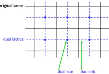
the dual links defined in Fig.1, wherethe solid lines represent the original square lattice and the

dashed

lines represent the dual lattice which is also square. The dual links correspond to the boundary of every neighboring spins.

Figure 1: Dual lattice of the $2d$ square lattice.

The domain wall variables thus reside

on

the dual links

as

shown in Fig.2. Spin

variables

are

$\sigma_{i}=\pm 1$ and domain wall variables are defined by $\alpha_{ij}=\sigma_{i}\sigma_{j}$, and it may

take two values: $\alpha=+1$ represents

no

domain wall and $\alpha=-1$ _represents the existence

of the domain wall.

Figure 2: Definition of domain walls.

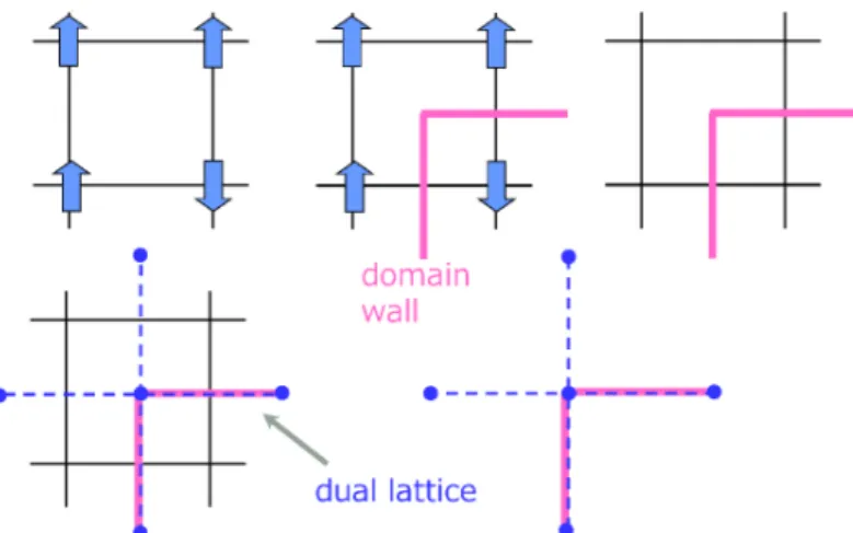
Anyspinconfiguration

can

be representedby

a

domain wall configuration. Asshown in

Fig.3,thedomain wallvariables

on

thefour links sharing asingledual site

are

determined

by four spins around it. We regard the final part of Fig.3

as

thedomain wall vertexdefined onthe dual site.

However, the correspondence between spins and domain wallsare not

one

to

one.

Tow spin configurations $\{\sigma_{i}\},$ $\{-\sigma_{i}\}$

are

mappedto the single domain wall configuration $\{\alpha_{ij}\}$

and this is two to one mapping. Therefore, although there

seems

to be no spontaneous symmetry breaking in the domain wall representation, its partition function or the free

energy has the exactly

same

singularities

as

the original spin partition function.

Figure 3: Domain wall representation of spin configuration.

The domain walls constitute the boundary of spin up or down domains, and therefore

the domain wall is conservative and makes topologically loop objects. Then the

non-conservative odd vertices as shown in Fig.4 are prohibited. $\prime$ 1 1 $–rightarrow$ 1 1 $\bullet/$

Figure 4: Prohibited non-conservative vertices.

Then wedefine the vertex tensor at each dual site, whichis a function of four domain wall variables around the dual site asshown in Fig.5. Sinceit has foursuffices, it is called the tensor.

$\alpha$

$T$

$T_{\alpha\beta\gamma\delta} \beta---|---\delta|$

$\gamma$

Figure 5: Vertex tensor.

The value of the vertex isdeterminedsothat the total product and the total summation withrespect tothe domain wall variables givethepartitionfunction of the original system

as

shown in Fig.6. The factor 2 at the top represents the two to one mapping nature of domain wall configuration versus spin configuration,

$\beta$

$Z=2$ $\sum T_{\alpha\beta\delta\gamma}T_{\delta\mu\nu\rho}\cdots$ $\alpha\beta\delta\gamma$

Figure 6: Partition function.

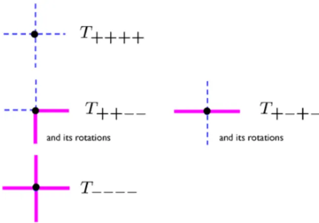
Therefore, the vertex value is proportional to the square root of the local statistical weight of the configuration. In caseof non-conservativevertex, the statistical weight must

vanish. Then the non-vanishing elements of this $2\cross 2\cross 2\cross 2$ tensor are only 8 elements

as

shown in Fig.7 1 $—+–\cdot T_{++++}$

1/’

$—\ulcorner_{and_{I}csro\iota at/ons}T_{++--}$ andits

$ro\iota z\iota j\circ nsT_{+-+-}$

Figure

7:

Non-vanishing elements oftensor.

3

Domain wall renormalization

group.

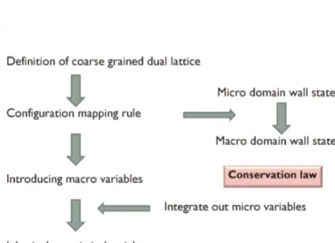
In this section we discuss how to define the renormalization group transformation in the domain wall representation, that is, renormalization of its vertex tensor $T$. The basic

strategy to define the renormalization group is flow-charted step by step in Fig.8.

According to this chart, first we define

coarse

graining ofthe dual lattice. We define

the coarse grained original lattice alaWilson [1], and then the

coarse

grained dual lattice is automatically defined

as

in Fig.9.

Note here that the

coarse

graining of original lattice keeps

a

half of their sites

com-monly, while the

coarse

graining of dual lattice has

no common

site

nor

link. In terms of

decimation, the

coarse

graining oflattice is obtained by decimation of sites, whereas the

coarse

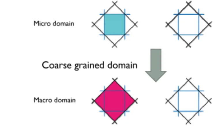
graining ofdual lattice is obtained by decimation of domains (dual plackets).

Then we define the

coarse

grained domain status

as

shown in Fig.10. Note that the

Definitionofcoarsegrained dual lattice

$Configuratio\cap l$

mapping rule

$-$

Micro domain$wa\ovalbox{\tt\small REJECT}\ovalbox{\tt\small REJECT}$

state

1.

1

Macro$doma/nwa\ovalbox{\tt\small REJECT}\ovalbox{\tt\small REJECT}$

state

’$ntroduc/ng$_macrovariables

$1$

$-$

integrateoutmicrovariables

Inherit the statistical weight:

Effective interactionsgiven byafunction ofmacrovariables

Figure 8: Domain wall renormalization group.

$arrow$ Decimating sites $arrow$ Decimating domains Figure 9: Coarse graining lattice and dual lattice.

The

coarse

grained domain status is just equal to the micro domain status at the center of it.

Figure 10: Definition ofcoarse grained domains.

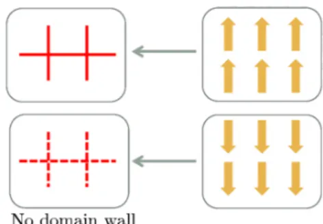
Next, the

coarse

grained domain walls

are

defined by the boundary of the

coarse

grained domains. Thus

we

get the mapping function from micro domain wall

configura-tion to the macro domain wall configuration. In Fig.11 we show the mapping function,

where the blue dual link denotes the micro domain wall and the red coarse grained dual

link denotes the macro

coarse

grained domain wall. The 4 configurations in the upper

row correspond to non-existence of the

macro

domain wall and those in the lower row

correspond to existence of the

macro

domain wall respectively. It is the eight to two

reduction mapping and this is the

coarse

graining of domain walls.

Figure 11: Macro domain walls and the mapping function.

It should be noted here that the

macro coarse

grained domain walls are boundary of

the

coarse

grained domains, and accordingly the

macro

domain walls are also conserved

by themselves.

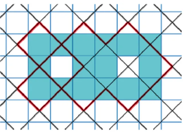
An example of the

coarse

graining ofdomain walls is shown in Fig.12. The left small island survives the

coarse

graining whereas the right

one

disappears.

Now the most non-trivial part

comes

up. We have defined the domain wall mapping

function between micro and

macro.

Thus the macro domain wall configuration must have

Figure 12:

Coarse

graining example.

domain wall configuration. And also the macro domain wall weight must be represented

by the renormalized tensor vertex. To make this procedure

we

learn from the tensor network renormalizationtechnique.

First of all, we split the micro domain

wa114-vertex

$T$ into

a

product of3-vertices $S$

as

shown in Fig.13, which is something like transforming the four-fermi interactions into

a pair of yukawa interactions by introducing auxiliary scalar fields. This decomposition is performed by the following matrix diagonalization,

$T=UDV$, (1)

where tensor $T$ is regarded as a matrix by grouping the domain wall indices as $T_{\{\alpha\beta\}\{\gamma\delta\}}$

and $U,$ $V$ are unitary matrices. The resultant matrix $D$ is a diagonal matrix of singular

values $\lambda_{M}$ which are all positive semi-definite. Then we can define $S$ as

$T_{\alpha\beta\gamma\delta}= \sum_{M}U_{\alpha\beta M}\sqrt{\lambda_{M}}\sqrt{\lambda_{M}}V_{M\gamma\delta}=S_{1\alpha\beta M}S_{2\gamma\delta M}$ , (2)

$S_{1\alpha\beta\Lambda I}=U_{\alpha\beta l1f}\sqrt{\lambda_{M}}, S_{2\gamma\delta M}\sqrt{\lambda_{M}}V_{M\gamma\delta}$ . (3)

Actually our $T$ matrix is

a

symmetric real matrix and it can be diagonalized by the

orthogonal transformation, that is, we have $S_{1}=S_{2}.$

$\alpha|$

$\alpha^{1}$

$-\beta+_{\wedge}\tau^{\delta}-(D^{rightarrow\beta\backslash _{M}^{S}}\backslash_{\gamma_{I}}s_{\delta-}$

–

Figure

13:

Splitting vertex $T$. Figure

14:

Renormalization

of

$T.$

We like to consider the scalar particle index $M$

as

the

macro

domain wall variable. Herewehave to do

some

approximation. Sincethe renormalized domain wall has only two

states naively, while the index $M$ has 4 degrees of freedomto satisfy theabove equation.

Then we adopt the approximation that only the relatively important channels should be

kept, that is, only two indices $M$ are taken among four. This is the approximation we have to do to define the domain wall renormalization group.

Next we integrate out all original domain wall indices $\alpha,$$\beta,$$\gamma,$ $\cdot$ and we get the effective weight function of$M$ at each

coarse

grained (renormalized) dual link, where $M$ is regarded

as

the renormalized domain wall variable. The effective weight

function

is written by the renormalized vertex tensor $T’$ defined by

$T_{MNKL}’= \sum_{\alpha\beta\gamma\delta}S_{\alpha\beta M}S_{\beta\gamma N}S_{\gamma\delta K}S_{\delta\alpha L}$ . (4)

Thisprocess is understandable

as

integrating out original fermion fields to leave effective

interactions among scalar fields, and it is graphically expressed in Fig.14.

The global landscape is drawn inFigs.15 and

16.

After therenormalizationprocedure, the renormalized dual lattice has $\sqrt{2}$ times larger spacing. This transformation can be

repeated and we have completed to define the domain wall renormalization group in the

lowest order approximation.

Figure 15: Global landscape 1. Figure 16: Global landscape 2.

The detailed analysis ofthis domainwall renormalizationgroup is foundin [5]. There,

the renormalization transformation is written down completely analytically and it is

proved that the physical selection of channels to interpret the renormalized indices as the macro domain wall variables is perfectly consistent with the optimized selection of largest singular values. Also the fixed point structure of the renormalization group flow

and the eigenvalues of the renormalization transformation around the fixed point are

calculated to give good values compared with the Onsager’s exact solution.

4

Introducing

the external

magnetic

field

So far, thereis

no

external field imposed, and

no

way of calculating magnetic quantities. In this section we propose

a

simple extension of the domain wall renormalization group

The domain wall representation is adegenerate descriptionof the spin configurations, that is, it does not discriminate $Z_{2}$ inverted spin configurations, $\{\sigma\}$ and $\{-\sigma\}$. To

discriminate these $Z_{2}$ inversion we introduce orientation of the domain wall as shown in Fig.17. Our rule here is that the up spin domainis

on

the right hand side of the oriented

domain wall when moving along thearrow. Simultaneously we doublethe no-domain wall

state and call them

as

up domain and down domain

as

in Fig.18. Now our domain wall

variable has four states at every dual link.

Figure 17: Oriented domain walls. Figure 18: Up domain and down domain.

$\S$ $\#$

updomain

$arrow\prime IlI$ $trightarrow\}$

Figure 19: Four domain wall states. Figure 20: $Z_{2}$ symmetry transformation.

The statistical weight is given by,

$\exp(K\sum_{<ij>}\sigma_{i}\sigma_{j}+h\sum_{i}\sigma_{i})$ (5)

where $\langle ij\rangle$

means

the nearest neighbor pair ofspins, _$K$

is the coupling constant and $h$ is

the external magnetic field. The four states of the domain wall variable on the dual link is diagrammatically expressed as in Fig.19. The $Z_{2}$ conjugate transformation is defined for these states as in Fig.20, which is important to understand the symmetry constraint of the vertex tensor and its renormalization transformation.

Now the indices $a,$ $\beta,$

$\gamma,$

$\delta$

of tensor $T$ takes 4 states each as in Fig.19, and tensor

$T_{\alpha\beta\gamma\delta}$ has originally $4^{4}=256$ elements. Only 16 elements are non-vanishing including rotation because of the domain wall conservation law with orientation, which

are

listed in Fig.21. In Fig.21, the barred variable

means

$Z_{2}$ conjugate, while $a=a,$ $c=\overline{c}$ are self $Z_{2}$ conjugate.

Thisdomain wallrepresentationhas 6dimensionalparameterspace$\{N, \overline{N}, b, b, a, c\}$ and

one

to

one

correspondence to spin interactions $\{C_{0}, K, K_{D}, K_{4}, h, h_{3}\}$, whose

$.–a^{1\underline{N}},^{--}1l$

$I_{I}\underline{\overline{b}}I^{--}I^{\cross 4}$

Figure 21: Non-vanishing

16

elements of the vertex tensor.

$+_{\sigma_{2}\sigma_{3}}^{\sigma_{1}\sigma_{4}}$

$\gamma$

$\gamma$

$- \beta\lrcorner^{\alpha}\ulcorner\delta$

Figure 22: Spin configuration. Figure

23:

2-dimensional matrix.

$\exp[C_{0}+K(\sigma_{1}\sigma_{2}+\sigma_{2}\sigma_{3}+\sigma_{3}\sigma_{4}+\sigma_{4}\sigma_{1})+K_{D}(\sigma_{1}\sigma_{3}+\sigma_{2}\sigma_{4})+K_{4}(\sigma_{1}\sigma_{2}\sigma_{3}\sigma_{4})$

$+h(\sigma_{1}+\sigma_{2}+\sigma_{3}+\sigma_{4})+h_{3}(\sigma_{1}\sigma_{2}\sigma_{3}+\sigma_{2}\sigma_{3}\sigma_{4}+\sigma_{3}\sigma_{4}\sigma_{1}+\sigma_{4}\sigma_{1}\sigma_{2})]$ (6)

Weuse 2-dimensionalmatrix representation$T_{\{\alpha\beta\}\{\gamma\delta\}}$ of$T_{\alpha\beta\gamma\delta}$

as

in Fig.23, and matrix

$T_{\{\alpha\beta\}\{\gamma\delta\}}$ is $16\cross 16$ dimensional. Actually, non-vanishing indices $\{\alpha\beta\}$ or $\{\gamma\delta\}$ are very

much and limited

as

shown in Fig.24. Only 8 elements are non-vanishing among 16

elements, and therefore $T_{\{\alpha\beta\}\{\gamma\delta\}}$ has only $8\cross 8$ non-vanishing block.

$z_{2}\downarrow \frac{t|}{---1\underline{|l}}I \lrcorner| \lrcorner t I^{\theta}$ $–\underline{S}_{r}| \underline{\mathfrak{g}_{I}^{I}l} \mathscr{Q}$

Figure 24: Non-vanishing indices.

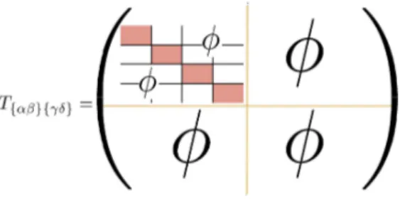
Considering the oriented domain wall conservationlaw, possiblecombination of indices

$\{\alpha\beta\}$ and $\{\gamma\delta\}$ are summarized in Fig.25. Thus the matrix $T_{\{\alpha\beta\}\{\gamma\delta\}}$ is divided into the

even

sectionand odd section and their $Z_{2}$conjugatesections. Each sectionconsists of$2\cross 2$

structure. Odd section and odd section

are

also constrained by the rotational symmetry. Accordingly, the total image of $T_{\{\alpha\beta\}\{\gamma\delta\}}$ takes the form shown in Fig.26. The matrix $T_{\{\alpha\beta\}\{\gamma\delta\}}$ is block diagonal consisting of 4 blocks of $2\cross 2$ each.

Now we set up the oriented domain wall renormalization group. The renormalized

domain wall states are defined by renormalized domain states. Then each sector

Even section $\overline{Even}$section

–

$Z_{2}$ Odd section $rightarrow$ $Z_{2}$

$\ovalbox{\tt\small REJECT}\ovalbox{\tt\small REJECT}$

–

rotation

Figure 25: Even and odd section.

wall interpretation through the renormalization procedure, we have to pick up one macro

channel each from every section.

Figure 26: Block diagonal matrix $T.$

Wediagonalize$T_{\{\alpha\beta\}\{\gamma\delta\}}$ as follows. Cosine and sinefunctions constituting the

orthog-onal matrices are denoted by $c_{a},$ $s_{a}$. Diagonalization ofeven sector is given by,

$(\begin{array}{ll}N bb c\end{array})=(\begin{array}{ll}c_{1} -s_{1}s_{1} c_{1}\end{array})(\begin{array}{ll}\lambda_{1} 00 \lambda_{2}\end{array})(\begin{array}{ll}c_{1} s_{1}-s_{1} c_{1}\end{array})$ (7)

$\overline{Even}$

section is expressed by usingthe $Z_{2}$ conjugate variables,

$(\begin{array}{l}\overline{N}\overline{b}\overline{b}\overline{c}\end{array})= (\overline{\frac{c_{1}}{s_{1}}} -\overline{\frac{S}{c_{1}}1})(\overline{\lambda_{1}0}\frac{0}{\lambda_{2}})(\begin{array}{ll}\overline{c_{1}} \overline{s_{1}}-\overline{s_{1}}\overline{c_{1}} \end{array})$ (8)

Odd and odd sections

are

parametrized by,

$(ab \frac{a}{b})=(\begin{array}{ll}c_{2} -\mathcal{S}_{2}s_{2} c_{2}\end{array}) (\begin{array}{ll}\lambda_{3} 00 \lambda_{4}\end{array})(\begin{array}{ll}c_{2} s_{2}-s_{2} c_{2}\end{array})$ (9)

where we adopt the following $Z_{2}$ conjugation rules,

Macro Up domain Odd section$|$ $rightarrow$ $Z_{l}$ $Z_{2}$ $rightarrow$ rotation $\overline{Even}$ section $-$

.

$\dot{c}_{\backslash }\backslash$ $\ddagger$

$\backslash \backslash$

$\backslash \backslash$

$\epsilon$

$\backslash \backslash \theta\cdot\blacksquare\cdot\cdot$

$-$

:

Macro Down domain

Odd section

Macro Domain Wall

Figure 27: Macro domain wall states.

Here larger eigenvalues (selected channels) in each section

are

taken tobe$\lambda_{1},$ $\overline{\lambda_{1}},$

$\lambda_{3},$ $\overline{\lambda_{3}},$ and they

are

also the 4largest singular values of

a118

singular values, which

assures

our

physical selection is consistent with the optimized singular value decomposition policy. The Feynman rules which couples micro and

macro

domain walls

are

listedin Fig.28. Domain walls

are

conserved in total for micro and

macro.

It shouldbe noted that they

are

oriented Feynman rulesand therefore they are irreversible, that is, the example diagrams

at the bottom of Fig.28 do not exist.

$\sqrt{\lambda_{1}}c_{1}$ $rightarrow^{Z_{2}}$ $===\Rightarrow$ $\sqrt{\overline{\lambda_{1}}}\overline{c_{1}}$ $\sqrt{\lambda_{1}}s_{1}$ $===\ll$ $\sqrt{\overline{\lambda_{1}}}\overline{s_{1}}$ $\sqrt{\lambda_{3}}c_{2}$ $\sqrt{\lambda_{3}}s_{2}$ $\sqrt{\lambda_{3}}s_{2}$ $\sqrt{\lambda_{3}}c_{2}$ e.g.

Figure

28:

Feynman rules between micro and

macro.

Renormalization transformation is carried out by calculating the one-loop diagrams

For example $a’$ and $c’$ keep $Z_{2}$ self conjugateness.

From the statistical weight defined in Eq.(5), the physical initial values of these 6

parameters are given by,

$N = e^{2K+h}\ovalbox{\tt\small REJECT}\overline{N}=e^{2K-h}$

$b = e^{h/2}rightarrow\overline{b}=e^{-h/2}$

$a = 1, c=e^{-2K}$ (11)

where left and right handed sides $ofrightarrow areZ_{2}$ conjugate to each other.

Now

we

write down the renormalization group transformation explicitly and analyti-cally as follows,

$\lambda_{1} = \frac{1}{2}(N+C+\sqrt{(N-C)^{2}+4b^{2}})$

$\overline{\lambda_{1}}= \frac{1}{2}(\overline{N}+C+\sqrt{(\overline{N}-C)^{2}+4\overline{b}^{2}})$

$\lambda_{3} = \frac{1}{2}(b-\overline{b}+\sqrt{(b-\overline{b})^{2}+4a^{2}})$

$t_{1} = \frac{1}{b}(\lambda_{1}-N) , t_{1}=\frac{1}{\overline{b}}(\overline{\lambda_{1}}-\overline{N}) , t_{2}=\frac{\lambda_{3}-b}{a},$

$c_{a}^{2}$ _$=$ $\frac{1}{1+t_{a}^{2}}$ $s_{a}^{2}=1-c_{a}^{2}$ , for $a=\{1, \overline{1}, 2\}$ (12)

Due to the$Z_{2}$ conjugate propertyof the totalsystem, there existsa4-dimensionalsubspace

of$Z_{2}$ invariant space,

$N=\overline{N}, b=\overline{b}, a, c$ , (13)

in which the renormalization group flows are confined. Therefore this subspace is

renor-malization group invariant subspace. The renormalization group transformation in this

$Z_{2}$ invariant subspace is exactly equal to what we have obtained previously [5].

We have to find the non-trivial fixed point to evaluate critical properties of the spon-taneous magnetization. Actually, however, there is no fixed point in the transformation in Eq.(12), since the vertex tensor $T$ continues to increase due to the volume effect of

the renormalization procedure which compensates the decimation of half of the degrees

of freedom at each renormalization step. We will set

some

normalization condition of$T$ and multiply a constant factor to all elements in $T$ to satisfy it at each renormalization step. This is called the gauge fixing since such constant multiplication does not change

any physical quantities of density type objects, such as, magnetization per site etc. The position of a fixed point itself depends on the gauge fixing condition adopted, called thegaugesimply. However, the eigenvalues around the fixed point does not depend

on the gauge. Here we show a proof of it briefly. We have two gauge fixing conditions, and coordinates on the gauge fixed manifolds are denoted by $x$ and $y$ respectively. There

are gauge transformation path (fiber bundle) in the total space on which $T$ is physically equivalent. This gauge transformation defines

a

relation between $x$ and $y,$

$+$ $=\lambda_{1}^{2}(c_{1}^{4}+s_{1}^{4})$

$Z_{2}\downarrow$

$a’=$

$+$

where $g$ is a non-singular function. Now the renormalization transformation are written

as

$x’=R_{1}(x) , y’=R_{2}(y)$, (15) and they have a fixed point at $x^{*}$ or $y^{*}$ satisfying,

$x^{*}=R_{1}(x^{*}) , y^{*}=R_{2}(y^{*}) , y^{*}=g(x^{*})$. (16)

The eigenvalues for $x$ and $y$ spaces are denoted by $\lambda_{1}$ and $\lambda_{2}$ respectively, and they are calculated to coincide with each other as follows,

$\lambda_{1} = R_{1}’(x^{*})=\frac{d}{dx}[g^{-1}(R_{2}(g(x^{*})))]=g^{-1/}(R_{2}(g(x^{*})))R_{2}’(g(x^{*}))g’(x^{*})$

$= g^{-1/}(y^{*})R_{2}’(y^{*})g’(x^{*})=R_{2}’(y^{*})=\lambda_{2}$ ₍₁₇₎

After the gauge fixing, the effective dimension ofthe total parameter space is five. In the $Z_{2}$ invariant 3-dimensional subspace

we

have found a non-trivial fixed point [5]. This

fixed point is also a fixed point in the tota15-dimensiona1 space. The eigenvalues around thefixed point consist of three $Z_{2}$

even

eigenvalues and two $Z_{2}$ odd eigenvalues.

We show transformation of variables between $\{C_{0}, K, K_{D}, K_{4}, h, h_{3}\}$ and domain

representations $\{N, \overline{N}, b, b, a, c\}$ in Fig.30, where letters in red are contributed by $Z_{2}$

odd interactions.

$Z_{2}\uparrow+C:\ N=\exp[C_{0}+2K+2K_{D}+K_{4}+h+4h_{3}]$

$\bullet\bullet\bullet 4\bullet \bullet\blacksquare \overline{N}=\exp[C_{0}+2K+2K_{D}+K_{4}-l\iota-4h_{3}]$

$i:[$

$+_{r*}^{11}$ $b= \exp[C_{0}^{\gamma}-K_{4}+\frac{h}{2}-2h_{3}]$ $Z_{2}\uparrow$ $\overline{b}=\exp[C_{0}-K_{4}-\frac{h}{2}+2h_{3}]$ $a=\exp[C_{0}-2K_{D}+K_{4}]$ $c=\exp[C_{0}-2K+2K_{D}+K_{4}]$

Figure

30:

Transformation between spin and domain wall interactions.

interactions $\{C_{0}, K, K_{D}, K_{4}, h, h_{3}\}$

are

given by,

$C_{0} = \frac{1}{16}\log[N\overline{N}a^{4}b^{4}\overline{b}^{4}c^{2}] K=\frac{1}{8}\log[N\overline{N}/c^{2}]$

$K_{D} = \frac{1}{16}\log[N\overline{N}c^{2}/a^{4}] , K_{4}=\frac{1}{16}\log[N\overline{N}a^{4}c^{2}/b^{4}\overline{b}^{4}]$

$h = \frac{1}{4}\log[Nb^{2}/\overline{N}^{2}\overline{b}^{2}] h_{3}=\frac{1}{16}\log[N\overline{b}^{2}/\overline{N}^{2}b^{2}]$ (18)

In the actual analysis oftherenormalization group flow, we set a gaugefixing condition,

$C_{0}=0$, that is, the spin independent factor is discarded.

5

Results

The $Z_{2}$

even

quantities suchasthefreeenergy, the specific heat and the correlation length

exponent have been reported previously [5]. Here

we

show $Z_{2}$ odd magnetic properties

only.

We plot typical high and low temperature flows in terms of the spin interaction pa-rameters in Fig.31 and Fig.32, where $n$ is the number of renormalization steps. In both

cases

only the single spin magnetic interaction $h$ survives at the infrared (macro) limit,

since we have to work with finite correlation length situation. The difference between

high and low temperatures is seen by the final enhancement factor of$h.$

$\subset 0$

$\overline{\alpha}$

$\cup 0\supset$

$0 5101520253035$

$n$

Figure 31: High temperature flow.

In Fig.33,

we

plotted the magnetization

versus

the initial nearest neighbor coupling constant $(\alpha\equiv e^{-2K})$ for various initial external magnetic fields. We

can see

the second order phase transition ofthe spontaneous magnetization around $\alpha=0.37036.$

Finally we evaluate renormalization group eigenvalues around the non-trivial fixed

point. We have three $Z_{2}$

-even

eigenvalues,

$\circ t$ $\underline{c}$ $\overline{\alpha}$ $\mathring{\cup}\supset$

$0 5101520253035$

$n$

Figure 32: Low temperature flow.

and two $Z_{2}$ odd eigenvalues,

{2.0214,

1.0547}.

(20)

The relevant $Z_{2}$

-even

eigenvalue gives the correlation length criticalexponent,

$\nu=\frac{\log\sqrt{2}}{\log 1.4224}=0.984$ _{, (21)}

which looksperfectcompared to the exact value of 1. Thepeculiar zeroeigenvalueappears because the renormalization group transformationin the $Z_{2}$

even

3-dimensional subspace

is actually constrained to be 2-dimensional. This seems an occasional constraint and no

physical significance is expected.

As for $Z_{2}$-odd eigenvalues, we encounter a serious deficit; there are two relevant

oper-ators. So far

we

have no good idea about how to cure this problem in this lowest order

formulation. Somenormalization issue owing to the singularity of decimation type

renor-malization group may be related. Ifwe use the larger eigenvalue to evaluate the magnetic susceptibilityexponent,we have

$\gamma=2.028$ , (22)

which looks not so good compared to the exact value of 7/4.

Wehave another idea of including the external magnetic field in the dualrepresentation

of the domain wall representation. Analysis of this dual renormalization group will be reported elsewhere [6].

Acknowledgments

We thank Yusuke Yoshimura for fruitful and critical discussion and comments, and

$\mathring{\underline{=c\varpi N}}$

$\dot{=oc\Phi\varpi}’$

Figure

33:

Magnetization

versus

temperature.

References

[1] L.P. Kadanoff, Physics. 2 (1966)

263.

K.

G.

Wilson, Rev. Mod. Phys. 47 (1975)

773

[2] M. Levin and C. P. Nave, Phys. Rev. Lett. 99 (2007)

120601.

[3] M. Hinczewski and A. N. Berker, Phys. Rev. E77 (2008)

011104.

[4] Z.-C. Gu, M. Levin andX.G. Wen, Phys. Rev. B78(2008)

205116

andarXiv:0806.3509

[cond-mat.str-el].

[5] K.-I. Aoki, Tamao Kobayashi and H. Tomita, Int.J.M.Phys.B23 (2009) 3739.

[6] K.-I. Aoki, Yasuhiro Fujii, Tamao Kobayashi, Daisuke Sato, Hiroshi Tomita and