A Cone Decomposition Method for Optimal Contribution Selection in Forest Tree Management (New Trends of Numerical Optimization in Advanced Information-Oriented Society)

A Cone Decomposition Method for Optimal Contribution Selection

in Forest Tree Management

Sena Safarina1 , Tim J. Mullin2 , and Makoto Yamashita1

1 Department of Mathematical and Computing Science, Tokyo Institute of Technology, 2‐12‐1‐W8‐29

Ookayama, Meguro‐ku, Tokyo 152‐8552, Japan.

2 The Swedish Forestry Research Institute (Skogforsk), Box 3, Sävar 91821, Sweden; and 224 rue du

Grand‐Royal Est, QC, J2M lR5, Canada.

1

Optimal Contribution Selection

In a forest tree management, one of essential phases for tree improvement is on recurrent cycles of selection. In that phase, genetic diversity is a main consideration for genetic gain performance in the

future. Therefore, an objective of optimal contribution selection (OCS) [1, S, 11,16] is to maximize

the genetic benefit under a genetic diversity constraint by determining the gene contribution from

each candidate.

This paper is concerned on OCS with an equal deployment problem (EDP) that designates a

specified number of selected individuals to have equally contribution to the gene pool; and it can

be formulated as:

maximize :

g^{T}x

subject to :

e^{T}x=1,

_{x_{i} \in\{0, \frac{1}{N}\}(i=1, \ldots, m),}

x^{T}Ax\leq 2\theta.

(1)

Here, the objective is to maximize the total benefit

g^{T}x

where

g=(g_{1}, g_{2}, \ldots, g_{m})^{T}

is the estimated

breeding values (EBVs) [7] representing the genetic value of candidates in the gene contribution

x\in \mathbb{R}^{m}_{, and} mis the total number of candidates. In this objective function, our decision variable

is xand we assume that _g is given. The first constraint e^{T}x=1 , with a vector of ones e\in \mathbb{R}^{m},

demands unity of the total contribution from all candidates. The second constraint

x_{i} \in\{0, \frac{1}{N}\}

interprets an equal contribution from each candidate, with N _{being the parameter to indicate the}

number of chosen candidates. Shortly speaking, N _{individuals has to be exactly chosen from a list}

of mavailable candidates in the EDP.

The last constraint in (1), x^{T}Ax\leq 2\theta , is our substantial constraint that requires a group

coancestry

\frac{x^{T}Ax}{2}

be under an appropriate level \theta>0. If the group coancestry

\frac{x^{T}Ax}{2}

is too high, the close relatedness among individuals in the population will decrease genetic diversity and also

impact on the reduction of long‐term genetic performance. The group coancestry [3] is computed

with the Wright numerator relationship matrix [15]

A\in \mathbb{R}^{m\cross m}

_{; and [12] emphasized that}

A

_is

always symmetric and semi‐definite positive.

In recent years, the OCS with EDP has been solved through a software package GENCONT [S]

which is an implementation based on Lagrange multipliers, but it forcibly fixes variables that exceed

though GENCONT generates a solution quickly, the solution is often suboptimal. To resolve this

difficulty in GENCONT, dsOpt, integrated in the software package OPSEL [9], was proposed by Mullin

and Belotti[ll]. Since dsOpt implements the branch‐and‐bound method combined with an outer

approximation method [4], dsOpt generates a very large number of subproblems in the framework

of branch‐and‐bound. This implementation is designed to acquire exact optimal solutions, but computing the solution takes a long time.

To deliver the problem in [8, 11], we consider to employ a second‐order cone form into the

quadratic constraint in 1. Utilizing Cholesky factorization of A _{so that}

_A=U^{T}U,

_{x^{T}Ax\leq 2\theta}

can be reformulated:

maximize :

_g^{T}x

subject to :

e^{T}x=1,

x_{i} \in\{0, \frac{1}{N}\}(i=1, \ldots, m),

(\sqrt{2\theta}N, Ux)\in \mathcal{K}^{m}

.

(2)

with

\mathcal{K}^{m}=\{(v_{0}, v)\in \mathbb{R}_{+}\cross \mathbb{R}^{m} : ||v||_{2}\leq v_{0}\}

is an

(m+1)

‐dimensional second‐order cone. However, non‐linearity arising from this second‐order cone also leads to a heavy computation cost.

In this paper, we examine and propose a cone decomposition method (CDM) that is based on

a geometric cut in a combination with a Lagrangian multiplier method and also draws on another form of second‐order cones. A cutting plane is a geometric cut if the plane is computed with an

orthogonal projection [2]. Cone decomposition itself has already been used in CPLEX which depends

on an outer approximation, therefore, the proposed CDM generates a different linear approximation. In addition, we prove that the Lagrangian multiplier method in the framework of CDM gives the analytical form for the geometric cut, therefore, the proposed CDM generates the linear cuts without relying on iterative methods.

The remainder of this paper is organized as follows. In Section 2, we propose the framework of CDM and demonstrates that the geometric cut in CDM has an analytical form. The numerical results will be presented in Section 3. Finally, in Section 4, we give some conclusions and discuss

future studies.

2

Cone Decomposition Method

In this section, we focus on the proposed cone decomposition method (CDM) for EDP (2) that

impose another form of second‐order cones as in the following corollary [13].

Corollary 2.1. A second‐order cone \mathcal{K}^{m} can be also written as

\mathcal{K}^{m}=\{(v_{0}, v)\in \mathbb{R}^{m+1}

: \exists w\in \mathbb{R}^{m} such that

v_{\dot{j}}^{2} \leq w_{j}v_{0}(j=1, \ldots, m),\sum_{j=1}^{m}w_{j}\leq v_{0}, v_{0}\geq 0\}.

Proof. Let

\hat{\mathcal{K}}^{m}

_{be {}

_{(v_{0}, v)\in \mathbb{R}^{m+1}}

_:

\exists w\in \mathbb{R}^{m}

s.t. v_{j}^{2}\leq w_{j}v_{0}(j=1, \ldots, m),

_{\sum_{j=1}^{m}w_{j}\leq v_{0},}

v_{0}\geq 0

}.

For

(\hat{v}_{0},\hat{v})\in\hat{\mathcal{K}}^{m}

, if \hat{v}_{0}=0 , then \hat{v}=0 _{due to the constraint}

_{\hat{v}_{j}^{2}\leq w_{j}\hat{v}_{0}}

_{, therefore, we know}

(\hat{v}_{0},\hat{v})\in \mathcal{K}^{m}

. In the case \hat{v}_{0}>0 , it holds that

_{\hat{v}_{0}\geq\sum_{\dot{j}=1}^{m}w_{j}\geq\sum_{\dot{j}=1}^{m}\hat{v}_{j}^{2}/\hat{v}_{0}}

, and this leads to

\hat{v}_{0}\geq\sqrt{\sum_{j=1}^{m}\hat{v}_{j}^{2}}.

Conversely, we take

(v_{0}, v)\in \mathcal{K}^{m}

. If v_{0}=0, we again have v=0; thus

(v_{0}, v)\in\hat{\mathcal{K}}^{m}

For positive v_{0}, we can use

w_{j}=v_{\dot{j}}^{2}/v_{0}

to show

(v_{0}, v)\in\hat{\mathcal{K}}^{m}

\square

Utilizing Corollary 2.1 and introducing new variable

y=Nx

to EDP (2) derives mixed‐integer

quadratic constraint problem (MI‐QCP):

maximize :

\frac{g^{T}y}{N}

subject to :

e^{T}y=N,

z=Uy

,

(3)

z_{i}^{2} \leq w_{i}c_{0}(i=1, \ldots, m), \sum_{\dot{i}=1}^{m}w_{i}\leq c_{0},y_{i}\in\{0,1\}(i=1, \ldots, m)

where z_{i}is the ith element of z,

c_{0}=\sqrt{2\theta N^{2}}

, and the decision variables of our new formulation are y, z, and w.

The nonlinear constraint in (3) is only the quadratic constraint

z_{i}^{2}\leq w_{i}c_{0}

with two variables

z_{i}

and w_{i}. In the proposed CDM, we generate the geometric cuts as cutting planes to these quadratic

constraint by employing orthogonal projections [2]. Therefore, the framework of the proposed CDM

is given as Algorithm 2.2.

Algorithm 2.2. [Cone decomposition method (CDM)]

Step 1 Let

P^{0}

_{be an MI‐LP problem that is generated from an optimization problem (3) by omitting}

the quadratic constraints

z_{i}^{2}\leq w_{i}c_{0}(i=1, \ldots, m)

. Apply an MI‐LP solver to P^{0}, and let its optimal solution be

(\hat{y}^{0},\hat{z}^{0},\hat{w}^{0})

. Let k=0.

Step 2 Let a set of generated cuts C^{k}=\emptyset.

Step 3 For each i=1, m, if

(\hat{z}_{i}^{k})^{2}\leq\hat{w}_{i}^{k}c_{0}

is violated, apply the following steps.

Step 3‐1 Compute the orthogonal projection of

(\hat{z}_{\dot{i}}^{k},\hat{w}_{i}^{k})

onto

_{z_{i}^{2}\leq w_{i}c_{0}}

by solving the following sub‐problem with the Lagrangian multiplier method;

minimize :

\frac{1}{2}(\overline{z}-\hat{z}_{\dot{i}}^{k})^{2}+\frac{1}{2}(\overline{w}-\hat{w}_{i}^{k})^{2}

(4)

subject to :

\overline{z}^{2}\leq\overline{w}c_{0}.

Let

(\overline{z}_{i}^{k},\overline{w}_{i}^{k})

be the solution of this subproblem. Step 3‐2 Add to C^{k}the following linear constraint

(\hat{w}_{ii}^{k_{-}\frac{i}{w}k}\hat{z}_{i}^{k}-\overline{z}^{k})^{T}(w_{i-}^{\frac{i}{w}k}z_{i}-\overline{z}_{i}^{k})\leq 0.

Step 4 If C^{k}is empty, output

\hat{y}^{k}

as the solution and terminate.

Step 5 Build a new MI‐LP P^{k+1} by adding C^{k}to P^{k} . Let the optimal solution of P^{k+1} be

(\hat{y}^{k+1},\hat{z}^{k+1},\hat{w}^{k+1})

.

Return to Step 2 with karrow k+1.

Step 3‐1 of Algorithm 2.2 computes the orthogonal projection. It would be desirable to compute the orthogonal projection on the original quadratic constraint

x^{T}Ax\leq 2\theta

, but such orthogonal

projection does not have an analytic form. A numerical method has been proposed in [6], but it

is an iterative method. Another iterative method is also proposed by [5] to solve different case

of second‐order cones. In contrast, the orthogonal projection in Step 3‐1 is onto a specific cone

\overline{z}^{2}\leq\overline{w}c_{0}

. The decomposition in Corollary 2.1 enables us to derive its analytical form, as proven in the following theorem.

Theorem 2.3. Assume that

(\hat{z},\hat{w})\in \mathbb{R}^{2}

violates

\hat{z}^{2}\leq\hat{w}c_{0}

. Let

(\overline{z},\overline{w})\in \mathbb{R}^{2}

be the orthogonal projection of

(\hat{z},\hat{w})

onto

z^{2}\leq wc_{0}

. Then,

(\overline{z},\overline{w})

can be given by an analytical form.

Proof. As in Step 3‐1 of Algorithm 2.2, the orthogonal projection

(\overline{z},\overline{w})\in \mathbb{R}^{2}

is the optimal solution

of the subproblem (4) that has a convex closed feasible region. Since

(\hat{z},\hat{w}) is outside of the region

z^{2}\leq wc_{0} , the optimal solution of (4) can be obtained with the following problem:

minimize :

\frac{1}{2}(z-\hat{z})^{2}+\frac{1}{2}(w-\hat{w})^{2}

(5)

subject to :

z^{2}=wc_{0}.

Next, we define a Lagrangian function of (5) with a Lagrangian multiplier \lambda\in \mathbb{R}_as:

\mathcal{L}(z, w, \lambda)=\frac{1}{2}(z-\hat{z})^{2}+\frac{1}{2}(w-\hat{w})^{2}-\lambda(wc_{0}-z^{2})

.

We consider \nabla \mathcal{L}=0in the Lagrangian multiplier method, therefore we obtain the conditions below

z-\hat{z}+2\lambda c_{0}=0;w-\hat{w}-\lambda c_{0}=0;-c_{0}w+z^{2}=0

that results in a following cubic function with respect to \lambda_:

4c_{0}^{2}\lambda^{3}+(4c_{0}^{2}+4c_{0}\hat{w})\lambda^{2}+(c_{0}^{2}+4c_{0}\hat{w})\lambda+(c_{0}\hat{w}-(\hat{z})^{2})=0.

When we apply Cardano’s Formula [14] to this cubic function, we obtain only one real root

\overline{A}.

This leads to \overline{z}=\hat{z}-2\overline{\lambda}c_{0} and \overline{w}=\hat{w}+\overline{\lambda}c_{0} . Therefore, the optimal solution (\overline{z},\overline{w}) of (4) has an

analytical form. \square

The termination of the proposed method is guaranteed by the following theorem. Theorem 2.4. Algorithm 2.2 terminates in a finite number of iterations.

Proof. Due to the binary constraints

y_{i}\in\{0,1\}

for i=1, m, the number of solution candidates

is at most 2^{m}_{. In the proposed method, we remove at least one candidate, therefore, the number}

of iterations is bounded above by 2^{m}. \square

3

Numerical Experiment

Numerical experiments were conducted for performance comparison of the proposed method CDM,

with the existing software dsOpt (as integrated in OPSEL) and GENCONT, and a general MI‐SOCP

solver CPLEX. We implemented CDM in MATLAB 9.3.0.713579 (R2017b) by setting CPLEX 12.71

as the MI‐LP solver. All numerical experiments were performed on Intel(R) Xeon(R) CPU E3‐1231

(3.40 GHz) and S GB memory space under 64‐bit Windows 10 operating system. The generated

data by the simulation POPSIM [10] were taken from https://doi.org/10.5061/dryad.9pn5m.

The sizes of the test instances are m=200_{, 1050, 2045, 5050, 10100, and 15222. We set parameter}

N=50,100, and as a stopping criterion for CPLEX, we used gap =1\%, 5%. The computation time

was limited to 3 hours for each execution.

Table 1 shows the results from the OCS solver GENCONT. In this table, the first, second, and third columns are the given parameter N_{, number of candidates} m_{, and} 2\theta_{. The columns}

g^{T}x

_”

Table 1: The result from GENCONT

N m 2\theta g^{T}x x^{T}Ax time (see)time \#chosen N

200 0.0334 11.472 0.03340 3.54 64 1050 0.0627 25.91 0.06270 7.20 81 50 2045 0.0711 438.36 0.07109 111.52 71 5050 0.1081 43.44 0.10810 1561.43 78 200 0.0258 8.89 0.02580 0.48 93 1050 0.0539 24.07 0.0539 4.77 94 100 2045 0.0628 432.75 0.06279 106.48 74 5050 0.0994 42.08 0.09940 1533.31 81

the computation time in the sixth column; and the number of chosen candidates (

\#

chosen

N

_{) by}

GENCONT in the last column. For a feasible solution x, it should hold

x^{T}Ax\leq 2\theta

and the number of

chosen candidate should be exactly N_{. However, the numerical result shows that \# chosen} N _did

not match the given N_{so that GENCONT failed to obtain feasible solutions. In addition, insufficient}

memory involved failure to output solution for m>5050.

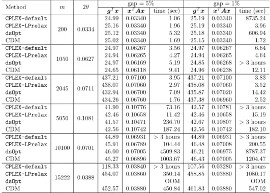
Tables 2 and 3 shows feasible solutions of the other methods for the given parameter N=50_and

N=100_{, respectively. Contrary to GENCONT, the number of chosen candidates of the rest methods}

match the given N. the first column displays different methods for our numerical experiment. In both tables, CPLEX‐default means that we used the default setting in CPLEX, and CPLEX‐LPrelax means that we explicitly set a parameter so that CPLEX used LP relaxation forcibly. We set the

time limit of 3 hours, and we indicate the violations of this time limit by >3_{hours’ and we used}

the best objective values in the 3 hours. In the case of out of memory, we used “OOM.”

CPLEX‐default shows its computation efficiency when the gap (the stopping criterion) is 5%.

On the other hand, for larger problems or smaller gaps, CPLEX‐default is more time‐consuming

than other methods. For instance, we can see a large time difference for the smallest size m=200.

CPLEX−default for gap 5% is the most efficient method among the seven methods, but it turns to be the slowest method when we set the gap as 1%. For such a tight gap, CPLEX‐LPrelax and

CDM can reduce computation time to less than 5 seconds. In the case m=15222_{, CPLEX‐default}

could not finish its computation within the time limit (three hours), and the best objective value

in the three hours was much worse than CPLEX‐LPrelax and CDM; CPLEX‐default only reached

g^{T}x=107.56.

From the difference between the results of CPLEX‐default and those of CPLEX‐LPrelax, we can infer that the default setting of CPLEX cannot solve EDPs efficiently, and we have to explicitly let

CPLEX know that LP relaxation is effective for EDPs.

Table 3 shows the results for the case N=100_{. Similar with the result in the previous table that}

CPLEX‐LPrelax and CDM obtain feasible solutions without having a memory problem. However, when our proposed method CDM is compared with CPLEX‐LPrelax, CPLEX‐LPrelax gives better

computation time performance than CDM for m\leq 10100. This is not only shown by Table 3,

but also it is on Table 2. For example, the computation time of CDM is 5 times slower than

CPLEX‐LPrelax to generate the solution of OCS with m=10100_{. Only for the largest size problem}

Table 2: Numerical comparison for EDPs

(N=50)

4 Conclusion and Future Work

In this study, we proposed the implementation of cone decomposition method to optimal contri‐ bution selection in forest tree management. The computation time problem difficulty from OPSEL makes us consider to propose the efficiency methods for solving OCS. We compared the efficiency

of our proposed implementation with the existing breeding selection software (GENCONT and OPSEL)

and also with the optimization solver CPLEX.

Based on the numerical result, we observed that our proposed relaxations, CDM still needs further improvement. It is seen by comparing CDM with CPLEX‐LPrelax that CDM can only give better performance than CPLEX‐LPrelax on the largest size problem. Therefore, in future study, we want to implement a sparsity structure on CDM so that it can reduce the computation time problem.

Acknowledgment

Table 3: Numerical comparison for EDPs

(N=100)

References

[1] J. Ahlinder, T. Mullin, and M. Yamashita. Using semidefinite programming to optimize unequal

deployment of genotypes to a clonal seed orchard. Tree genetics ty genomes,

10(1):27-34

, 2014.

[2] P. Bialoń. Some variants of projection methods for large nonlinear optimization problems.

Journal of Telecommunications and Information Technology, pages 43‐49, 2003.

[3] C. C. Cockerham. Group inbreeding and coancestry. Genetics, 56(1):89 , 1967.

[4] M. A. Duran and I. E. Grossmann. An outer‐approximation algorithm for a class of mixed‐

integer nonlinear programs. Mathematical programming,

36(3):307-339

, 1986.

[5] O. Ferreira and S. Németh. How to project onto extended second order cones. Journal of

Global optimization,

70(4):707-71S,

201S.

[6] Y. N. Kiseliov. Algorithms of projection of a point onto an ellipsoid. Lithuanian Mathematical

Journal,

34(2):141-159

, 1994.

[7] M. Lynch and B. Walsh. Genetics and analysis of quantitative traits. Sinauer Sunderland, MA,

[S] T. H. Meuwissen. GENCONT: an operational tool for controlling inbreeding in selection and

conservation schemes. In Proceedings of the 7th Congress on Genetics Applied to Livestock Production, pages 19‐23, 2002.

[9] T. J. Mullin. OPSEL 2.0: A computer program for optimal selection in tree breeding. Arbet‐

srapport fr\mathring{a}nSkogforsk Nr 954‐2017, Skogforsk, Uppsala, SE, 2017.

[10] T. J. Mullin. Popsim: a computer program for simulation of tree breeding programs over

multiple generations. Arbetsrapport fr\mathring{a}n Skogforsk Nr. 984‐2018, Skogforsk, Uppsala, SE, 2018.

[11] T. J. Mullin and P. Belotti. Using branch‐and‐bound algorithms to optimize selection of a

fixed‐size breeding population under a relatedness constraint. Tree genetics g genomes,

12(1):4,

2016.

[12] R. Pong‐Wong and J. A. Woolliams. optimisation of contribution of candidate parents to

maximise genetic gain and restricting inbreeding using semidefinite programming (open access

publication). Genetics Selection Evolution, 39(1):3 , 2007.

[13] J. P. Vielma, I, Dunning, J. Huchette, and M. Lubin. Extended formulations in mixed integer

conic quadratic programming. Mathematical Programming Computation,

9(3):369-418

, 2017.

[14] R. Witula and D. Slota. Cardano’s formula, square roots, chebyshev polynomials and radicals.

Journal of Mathematical Analysis and Applications,

363(2):639-647

, 2010.

[15] S. Wright. Coefficients of inbreeding and relationship. The American Naturalist,

56(645):330-338, 1922.

[16] M. Yamashita, T. J. Mullin, and S. Safarina. An efficient second‐order cone programming

approach for optimal selection in tree breeding. optimization Letters, 12(7):1683−1697, 2018.