Dynamics of entire functions with two singular values (Complex Dynamics)

(1)

Dynamics

of

entire

functions with

two

singular

values

Shu

nsuke MOROSAWA

Department

of

Mathematics and Information

Science,

Faculty

of

Science,

Kochi

University

and

Masahiko

TANIGUCHI

Graduate School of

Science, Kyoto University

1 Introduction

Form the structural viewpoint, the simplest entire function is a quadratic

polynomial. It has two critical points. One is the point at infinity and is

always asuperattracting fixed point. Hence the behavior of the finite critical

point decides the dynamics onthe complex plain. In this sense, dynamics of

cubic polynomialis decided by twofinite critical points. The family of cubic

polynomials has been investigated by several authors (e.g. [2], [3] and [4]).

In this note, we treat three simplest kinds of entire functions having only

two singular values. They are structurally finite entire functions, which are

definedby Taniguchi in [9].

Definition

1. Cubic (monk centered) polynomials

$P_{a,b}(z)=z^{3}-3a^{2}z+b$.

The critical points are$\pm a$, and the singular (critical) values are$b\mp 2a^{3}$.

We denote by $\mathrm{P}\mathrm{o}1\mathrm{y}_{3}$ the family consisting ofall cubic polynomials.

2. Simply decorated exponential functions

$E_{a,b}(z)=a(z+b)e^{z}$ $(a\neq 0)$.

The single critical point is $-b-1$, and the singular values are 0 and

$-a\exp(-b-1)$. Wedenote by$\mathrm{D}\exp_{1}$ thefamily consistingof allsimply

(2)

3.

Complex

error

functions

$C_{a,b}(z)=a \int_{0}^{z}e^{-t^{2}}dt+b$ $(a\neq 0)$.

The singular values

are

$\pm aA+b$ with $A^{2}=\pi/4$. We denote by Cerf

the family consisting of all complex error functions.

Definition We denote by

_S2

the union of the families $\mathrm{P}\mathrm{o}1\mathrm{y}_{3}$, $\mathrm{D}\exp_{1}$ and

Cerf.

The second family has been investigated by Morosawa ([5] and [6]) and

others. But the third family

seems

to have been paid almost no attentions.

Recently, Morosawa and Taniguchi obtain

some

results on complex error

functions (see, [10], [7] and [11]).

2 Classification

of

hyperbolic

Fatou

compo-nents

Let $f$ be a Speiser function, i.e.

a

function having only a finite number of

singular values, and $\langle$ be an asymptotic value of $f$ in the Fatou set $F(f)$ of

$f$. Then there exists an asymptotic path for

4

in $F(f)$. The Fatou

compo-nent containing such

a

path is called a prelusive component of $f$ for $\langle$

.

The

Fatou component containing a critical point $c$ of$f$ is also called a prelusive

componentfor the criticalvalue $f(c)$.

Note that a singular value may have several prelusive components for it.

The following Proposition is well-known.

Proposition 1 The immediate basin

_for

an attracting cyclic contains at

least

one

prelusive component.

We say that aSpeiser function $f$ is hyperbolicif the orbit of every singular

value of $f$ belongs to basins of attracting periodic points. In the

case

of

hyperbolic entire functions in $S_{2_{7}}$ there

are

four kinds of dynamics (cf. [4],

[8]$)$

.

Definition We say that a hyperbolic function

f

$\in \mathcal{X}$, where $\mathcal{X}=\mathrm{P}\mathrm{o}1\mathrm{y}_{3}$,

$\mathrm{D}\exp_{1}$ or Cerf is

1.

_of

adjacent type if there exists a prelusive component $U$ for both of

singular values and there exists the smallest positive integer $p$ such

that

$f^{p}(U)\subseteq U$,

(3)

2.

_of

bitransitive type ifthere exist different prelusive components $U_{1}$ and $U_{2}$ and the smallest positive integers $p$ and $q$such that

$f^{\mathrm{p}}(U_{1})\subset U_{2}$, $f^{q}(U_{2})\subseteq U_{1}$,

and

we

denote the set of all such $f$ with fixed $p$ and $q$ by $B_{p+q}=$

$B_{p+q}(\mathcal{X})$,

3.

_of

captured type if there exist two prelusive components $U_{1}$ and $U_{2}$ and

the smallest non-negative integers $p$, $q$, and $t$ such that $U_{1}$ is disjoint

from $\bigcup_{k=0}^{\infty}f^{k}(U_{2})$, $t\geq 1$ with

$f^{t}(U_{1})\cap(_{k=0}^{\infty}\cup f^{k}(U_{2}))\neq\emptyset$

and, $p\geq 0$ and $p+q\geq 1$ with

$f^{t+p}(U_{1})\subset U_{2}$, $f^{p+q}(U_{2})\subseteq U_{2}$,

and we denote the set of all such $f$ with fixed $p$,$q$,$t$ by $C(t)p+q=$

$C_{(t)p+q}(\mathcal{X})$, and

4.

_of

disjoint type ifthere exist two prelusive components $U_{1}$ and $U_{2}$ and

the smallest positive integers $p$ and $q$ such that

$f^{p}(U_{1})\subset U_{1}$, $f^{q}(U_{2})\subset U_{2}$,

and

$k=0k=0\cup f^{k}(U_{1})\cap\cup f^{k}(U_{2})=\emptyset\infty\infty$,

and

we

denote that the set of all such $f$ with fixed$p$ and $q$ by $D_{p,q}=$

$D_{p,q}(\mathcal{X})$.

Bergweiler [1] pointed out the following.

Theorem 2

_if

a

_forward

invariant Fatou component U

_of

a

Speiser

_function

f

contains all the singular values

_of

f, then U is completely invariant

Corollary 1 The set $C_{(1)0+1}=C_{(1)0+1}(\mathcal{X})$, where $\mathcal{X}=\mathrm{P}\mathrm{o}1\mathrm{y}_{3\mathrm{r}}$ $\mathrm{D}\exp_{1}$ or

Cerf, is empty.

show a criterion for ahyperbolic function being ofcapture type.

Theorem 3 Let $f$ be a hyperbolic

function

belonging to $\mathrm{P}\mathrm{o}1\mathrm{y}_{3}$ or Dexpj,

Assume

$f$ has a superattracting

fixed

point $\zeta_{1}$. Let $\zeta_{2}$ be another singular

value.

_if

there exists

some

$N>0$ satisfying $f^{N}(\zeta_{2})=\zeta_{1;}$ then$f$ is

of

capture

(4)

3 Examples

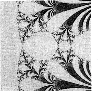
Example 1 Let

$E_{-1,-1}(z)=-(z-1)e^{z}$

.

Then $E_{-1,-1}$ is hyperbolic and belongs to $C_{\langle 1)0+2}$

.

Verification.

The function has a critical point 0 and a singular value 0.

Since $f(0)=1$ and $f(1)=0_{1}$ it has a superattracting cycle with period two.

Hence it is hyperbolic. By using a graphical analysis, we can find a fixed

point $x\in$ $(0, 1)$ and it is easy to

see

that it is repelling. Hence there exists a

point in $(-\infty, 0)$ which is mapped

on

$x$. Since the Fatou set of $E_{-1,-1}(z)$ is

symmetric with respect to the real axis, the prelusive component for 0 does

not contain 0.

Figure 1: The Julia set of $E_{-1,-1}$. The range shown is $|\Re z|<2.4$ and

$|_{S}^{\alpha}z|<2.4$.

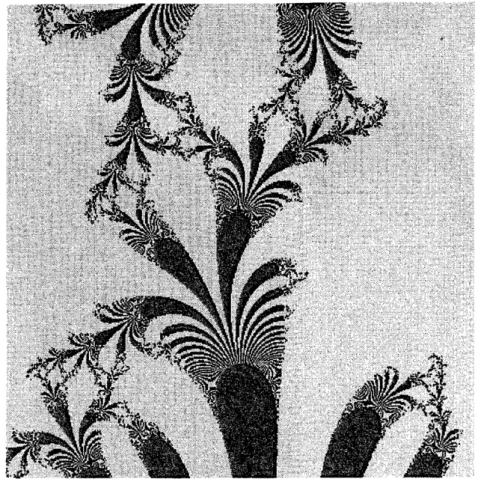
Example 2 Assume $a$ and $b$ satisfy

ab $=$ $-b-1$ $be^{b+1}$ _$=$ -1.

Then $E_{a}$_,$b$ is hyperbolic and belongs to $C_{(2)0+1}$

.

In this case, the prelusive

component

_for

the asymptotic value is captured by the prelusive component

(5)

Verification.

The first equation implies $-b-1$ is a superattracting fixed

point. Thesecond implies $E_{a,b}(0)=-b-1$. Prom Theorem 3, we obtain the

claim.

Figure 2: The Julia set of $E_{a,b}$, where $a=-0.952639\cdots+$i0.114414$\ldots$ and

$b=-3.08884\cdots+$i7.46149$\ldots$ which satisfy the equation$1\mathrm{S}$ in Example 2. It

has asuperattracting fixed point 2.08884$\ldots-$i7.46149$\ldots$ . The range shown

is $-7<\Re z<3$ and $-8<sz\triangleright<2$_.

Example 3 Assume a and b satisfy

$a$ $=$ $\frac{1}{1+2b}$

$\frac{1}{1+2b}-2b\exp(\frac{3}{2}+b)$ $=$

0.

Then $E_{a}$_,$b$ is hyperbolic and belongs to $C_{(2)0+1}$. In this case, the prelusive

component

_for

the critical value is captured by the prelusive component

_for

the asymptotic value.

Verification.

The first equation implies 1/2 is anattracting fixed point. The

(6)

Figure 3; _The Julia set of $E_{a,b}$, where $a=$

-0.0605096

– and $b=$

-5.51185 $\ldots$ which satisfythe equations in Example 3. It has

an

attracting

fixed point 1/2. The range shown is $-2<\Re z<6$ and $|\Leftrightarrow sz|<3$.

Example 4 Let

$C_{a,b}(z)=a \int_{0}^{z}e^{-w^{2}}dw+b$,

with $a=1.41055+\mathrm{i}1$,23448 and $b=-0.121077-$ 20.8811. Then it belongs to $C_{(2)0+1}$.

References

[1] W. Bergweiler, oral communications.

[2] B. Branner, The parameter space

for

cubic polynomials, Chaotic

Dy-namics and Fractals, Academic Press, (1996),

169-179.

[3] B. Branner and J. Hubbard, The iteration

of

cubic polynomials, Part I:

Acta Math. 160, (1988),

143-206.

Part ILActaMath. 169,

(1992),229-325.

[4] J. Milnor, Remarks

on

iterated cubic maps, Experimental Math. $1_{7}$

(7)

Figure 4: The Julia set of$C_{a,b}$. Ithas an attractingfixed point

0.8910492

\cdots

-i0.0372985\cdots. Its asymptotic values are $a_{1}=1.12899$\cdots --i0.2129294$\cdots$

and $a_{2}=-1.371144$\cdots -i1.975129\cdots . The immediate basin is the prelusive

component for $a_{1}$ and $C_{a,b}^{2}(a_{2})$ is contained in it. The range shown is $-2.3<$

$\Re z<1.7$ and $-2.4<\triangleright sz$ _$<1.6$.

[5] S. Morosawa, Note on the iteration

_of

$f_{\ell\iota}(z)=z\exp(z+\mu)$, Sci. Bui.

Josai. Univ., Special Issue 4(1998), 11-16.

[6] S. Morosawa, Local connectedness

_of

Julia sets

_for

transcendental

en-tirc functions, Proceedings of the International Conference

on

Nonlin-ear

Analysis and Convex Analysis (eds. W. Takahashi and T. Tanaka),

World Scientific, November 1999,

266- 273.

[7] S. Morosawa, Fatou components whose boundaries have a

common

(8)

[8] M. Rees, Components

_of

degree two hyperbolic rational maps, Invent.

Math. 100, (1990),

357-382.

[9] M. Taniguchi, Maskit surgery

_of

entire functions, RIMS Kokyuroku

1220, (2001),

7-16.

[10] M. Taniguchi, Synthetic

_defor

mation spaces

_of

an

entire function,

Con-temporary Math,, 303, (2002),

107-136.

[11] M. Taniguchi, Geometric compactification

of

synthetic

_deformatio

$n$