A dynamical System Approach to Coding Theory : Rational Maps and Maximum Likelihood Decodings (Dynamical Systems : Theories to Applications and Applications to Theories)

A dynamical

System

Approach

to Coding Theory:

Rational

Maps and

Maximum

Likelihood Decodings

Kazunori

Hayashi

*

Yasuaki

Hiraoka

\dagger

Abstract

Thisarticlesurveys arecent preprint [1], which studies maximumlikelihood(ML)

decod-ing in error-correcting codes as rational maps and proposes an approximate ML decoding

rule by usingaTaylor expansion. The point for the Taylor expansion, which will bedenoted

by$p$in the paper, is properly chosen byconsideringsomedynamical systemproperties. We

havetwo results about this approximate ML decoding. The first resultprovesthat the order

of thefirst nonlinear termsin the Taylorexpansion isdeterminedby theminimum distance

ofits dual code. As the second result, we give numerical results on bit error probabilities

for the approximate ML decoding. These numerical results show better performance than

that of BCH codes, and indicate that this proposedmethod approximates the original ML

decoding very well.

1

Communication

Systems

Amathematical modelof communication system in information theory

was

developed by

Shan-non

[3]. A general block diagram for visualizing the behavior ofsuch systems is given by

Fig-ure

1.1. The

source

transmits

a

k-bit message $m=(m_{1}\cdots m_{k})$ to the destination via the

channel, which is usually affected by noise $e$

.

In order to

recover

the transmitted message

at the destination under the influence of noise,

we

transform the message into

a

codeword

$x=(x_{1}\cdots x_{n}),$ $n\geq k$, by

some

injective mapping $\varphi$ at the encoder and input it to the

chan-nel. Then the decoder transforms

an

n-bit received

sequence

ofletters $y=(y_{1}\cdots y_{n})$ by

some

decoding mapping $\psi$ in order to obtain the transmitted codeword at the destination. Here

we

consider all arithmeticcalculations in

some

finitefield and in this paper

we

fix it

as

$F_{2}=\{0,1\}$

.

As

a

model of channels,

we

deal with

a

binary symmetric channel (BSC) in this paperwhich

is characterized by the transition probability $\epsilon(0<\epsilon<1/2)$. Namely, with probability $1-\epsilon$, the output letter is

a

faithful replica of the input, and with probability $\epsilon$, it is the opposite of

the input letter for each bit (see Figure 1.2). In particular, this is

an

example of memoryless

channels.

Then,

one

ofthe main purposes of coding theory is to develop

a

good encoder-decoder pair

$(\varphi, \psi)$ which is robust to noise perturbations. Hence, the problem is how

we

efficiently

use

the

redundancy $n\geq k$ in this setting. $*$

Kyoto University: kazunoriQi.kyoto-u.ac.jp

$x_{i}=0$ $1-\epsilon$ $y_{i}=0$

Figure 1.1: Communication system

2

Linear Codes

$x_{t}=1$ $1-\epsilon$ _{$y_{i}=1$}

Figure 1.2: Binary synunetric channel

A code with a linear encoding map $\varphi$ is called a linear code. A codewol$d$ in a linear code can

be characterized by its generator matrix

$G=(\begin{array}{lll}g_{11} \cdots g_{1n}| \ddots |g_{krl} \cdots g_{kn}\end{array})=(g_{1}\cdots g_{n})$

.

$g_{i}=(\begin{array}{l}g_{1i}|g_{ki}\end{array})$ , $i=1,$ _$\cdots,$$n$,

where each element $g_{ij}\in F_{2}$

.

Therefore the set ofcodewords is given by

$C=\{(x_{1}\cdots x_{n})=(m_{1}\cdots m_{k})G|m_{i}\in F_{2}, \}$

.

$\beta C=2^{k}$.

Here without loss of generality,

we

assume

$g_{i}\neq 0$ for all $i=1,$$\cdots.n$ and rank $G=k$. We call

$k$ and _$n$ the dimension and the length ofthe code, respectively.

Because of the linearity, it is also possible to describe $C$

as

a kernel of a matrix $H$ whose

$m=n-k$ row vectors are linearly independent and orthogonal to those of$G$, i.e.,

$C=\{(x_{1}\cdots x_{n})|(x_{1}\cdots x_{n})H^{t}=0\}$

.

$H=(\begin{array}{lll}h_{l1} \cdots h_{1r\prime}| \ddots |h_{n|1} \cdots h_{mn}\end{array})=(h_{1}\cdots h_{n})$,

where $H^{t}$

means

the transpose matrix of _$H$. This matrix _$H$ is called

a

parity check matrix of

$C$

.

The dual code$C^{*}$ of$C$ is defined in such

a

way that

a

paritycheck $1nat_{I}\cdot ix$of$C^{*}$ is given by

a

generator matrix $G$ of$C$

.

The$H\prime e1\ln\dot{m}ng$ distance$d(x, y)$ betweentwo n-bit sequences $x.y\in F_{2}^{n}$ is given by the nulnber

of positions at which the two sequences differ. The weight ofanelement $x\in F_{2}^{n}$ isthe Hamming distance to $0$

,

i.e.. _$d(x)$ $:=d(x, 0)$

.

Then the minimum distance _$d(C)$ of a code $C$ is defined by

two different ways

as

$d(C)= \min\{d(x_{i}y)|x.y\in C$ aand $x \neq y\}=\min\{d(x) 0\neq x\in C\}$

.

Hel$e$ the second equality results from the linearity. It is easy to observe that the $mini_{1}nu\ln$

distance is $d(C)=d$ if and only if there exists aset of$d$ linearly dependent column vectors of$H$

but no set of$d-1$ linearly dependent coluinn vectors.

For

a

code $C$ with the minimum distance $d=d(C)$ , let

us

set $t$ _{$:=\lfloor(d-1)/2\rfloor$}, where $\lfloor a\rfloor$ is

the integer part of$a$

.

Then, it follows from the followingobservation that $C$

can

correct $t$

errors:

if$y\in F_{2}^{n}$ and $d(x, y)\leq t$ for

some

$x\in C$ then $x$ is the only codeword with $d(x, y)\leq t$

.

In this

sense.

the minimunz distance is

one

of the import,ant parameters to $me\Re^{\neg}U1^{\backslash }e$performance of a

3

Maximum Likelihood

Decoding

Let us recall that, given a transmitted codeword $x$, the conditional probability $P(y|x)$ of a

received sequence $y\in F_{2}^{n}$ at the decoder is given by

$P(y|x)=P(y_{1}|x_{1})\cdots P(y_{n}|x_{n})$

for

a

memoryless channel. Maximum likelihood(ML) decoding$\psi$ : $F_{2}^{n}\ni y\mapsto\tilde{x}\in \mathbb{F}_{2}^{n}$ is given by

takingthe marginalization of$P(y|x)$ foreach bit. Precisely speaking, for

a

received sequence $y$,

the i-th bit element $\tilde{x}_{i}$ ofthe decoded word $\tilde{x}$ is determined by the following rule:

$\tilde{x}_{i}:=\{\begin{array}{l}1, \sum_{x\in C}P(y|x)\leq\sum_{x\in C}P(y|x)x_{i}=0x_{i}=1, i=1, \cdots, n.0, otherwise\end{array}$ (3.1)

In general, for

a

given decoder $\psi$, the bit

error

probability _{$P_{bit}^{e}= \max\{P_{1}^{e}, \cdots, P_{n}^{e}\}$}, where

$P_{i}^{e}= \sum_{x\in C,y\in \mathbb{F}_{2}^{n}}P(x, y)(1-\delta_{x_{i},\overline{x}_{i}})$, $\tilde{x}=(\tilde{x}_{1}, \cdots,\tilde{x}_{n})=\psi(y)$,

$\delta_{a,b}=\{\begin{array}{l}1, a=b0, a\neq b’\end{array}$

is

one

ofthe important

measures

of decoding performance. Obviously, it is desirable to design

an encoding-decoding pair whose bit

error

probability is

as

small

as

possible. It is known that

ML decoding attains the minimum bit

error

probability for any encodings under the uniform

distribution

on

$P(x)$. In this sense, ML decoding is the best for all decoding rules. However

its computational cost requires at least $2^{k}$ operations, and it is too much to

use

for practical

applications.

From the above property of ML decoding, one of the key motivation of this work

comes

from the following simple question. Is it possible to accurately approximate the ML decoding

rules with low computational complexity? The main results in this paper give

answers

to this

question.

4

Main Results

Let

us

first define for each codeword $x\in C$ its codeword polynomial $F_{x}(u_{1}, \cdots, u_{n})$

as

$F_{x}(u_{1}, \cdots, u_{n}):=\prod_{i=1}^{n}\rho_{i}(u_{i})$, $\rho_{i}(u_{i})=\{\begin{array}{ll}u_{i}, x_{i}=1,1-u_{i}, x_{i}=0.\end{array}$

Then

we

define

a

rational map $f$ : $I^{n}arrow I^{n},$ $I=[0,1]$, by using codeword polynomials

as

$f:(u_{1}, \cdots, u_{n})\mapsto(u_{1}’, \cdots, u_{n}’)$,

$u_{i}’=f_{i}(u):= \frac{\sum_{x\in C,x_{i}=1}F_{x}(u)}{H(u)}$, $i=1,$_{$\cdots,$ $n$},

$H(u):= \sum_{x\in C}F_{x}(u)$, (4.1)

where $u=(u_{1}, \cdots, u_{n})$

.

This rational map plays the most important role in the paper. It is

For

a

sequence $y\in F_{2}^{n}$, let

us

take

a

point $u^{0}\in I^{n}$ as

$u_{i}^{0}=\{\begin{array}{ll}\epsilon, y_{i}=01-.\epsilon, y_{i}=1’\end{array}$ $i=1,$

$\cdots,$ $n$, (4.2)

where $\epsilon$ is the transition probability of the channel. Then it is straightforward to check that

$F_{x}(u^{0})=P(y|x)$. Namely, the conditional probability of $y$ under

a

codeword $x\in C$ is given

by the value of the corresponding codeword polynomial $F_{x}(u)$ at $u=u^{0}$

.

Therefore, from the

construction ofthe rational map, ML decoding (3.1) is equivalently given by the following rule

$\psi:F_{2}^{n}\ni y\mapsto\tilde{x}\in F_{2}^{n}$,

$\tilde{x}_{i}=\psi_{i}(y):=\{\begin{array}{l}1, f_{i}(u^{0})\geq 1/20, f_{i}(u^{0})<1/2’\end{array}$ $i=1,$

$\cdots,$ $n$

.

(4.3)

In this

sense, the

studyof ML decoding

can

betreated by analyzing the image

of

the initialpoint

(4.2) by the rational map (4.1). Some of the properties of this map in the

sense

of dynamical

systems and coding theory is studied in detail in [1].

For the statement of the main results, we only here mention that this rational map has

a

fixed point $p:=(1/2, \cdots, 1/2)$ for any generator matrix (Proposition 2.2 in [1]). Let us denote

the Taylor expansion at$p$ by

$f(u)=p+Jv+f^{(2)}(v)+\cdots+f^{(l)}(v)+O(v^{l+1})$_{, (4.4)}

where$v=(v_{1}, \cdots, v_{n})$is avectornotation of$v_{i}=u_{i}-1/2,$$i=1,$$\cdots,$$n,$ $J$is the Jacobi matrix at

$p,$ $f^{(i)}(v)$ corresponds to the i-th order term, and $O(v^{l+1})$ means the usual order notation. The

reason

why we choose $p$

as

the approximating point is related to the local dynamical property

at $p$ and is discussed in [1].

By truncating higher oder terms $O(v^{l+1})$ in (4.4) and denoting it

as

$\tilde{f}(u)=p+Jv+f^{(2)}(v)+\cdots+f^{(l)}(v)$_,

we can define the l-th approximation of ML decoding by replacing the map $f(u)$ in (4.3) with

$f(u)$_{, and denote this approximate ML decoding by} $\tilde{\psi}$ :

$F_{2}^{n}arrow F_{2}^{n}$, i.e.,

$\tilde{\psi}:F_{2}^{n}\ni y\mapsto\tilde{x}\in F_{2}^{n}$,

$\tilde{x}_{i}=\tilde{\psi}_{i}(y):=\{\begin{array}{l}1, \tilde{f_{i}}(u^{0})\geq 1/20, \tilde{f_{i}}(u^{0})<1/2’\end{array}$ $i=1,$

$\cdots,$$n$. (4.5)

Let

us

remark that the notations $\tilde{f}$ and $\tilde{\psi}$ do not explicitly express the dependence

on

$l$ for

removing unnecessary confusions of subscripts.

4.1

Duality

Theorem

We note that there

are

two different viewpoints on this approximate ML decoding. One wayis

that, inthe

sense

ofits precision, it is preferable to haveanexpansion with large $l$. On the other

hand, fromthe viewpoint of low computational complexity, it is desirable to include many

zero

elements in higher order terms. The next theorem states

a

sufficient condition to satisfy these

Theorem 1 Let $l\geq 2$

.

If

any distinct $l$ column vectors

of

a genemtor matrix $G$

are

linearly

independent, then the Taylor expansion (4.4) at$p$

of

the mtional map (4.1) takes the following

$fom$

$f(u)=u+f^{(l)}(v)+O(v^{l+1})$_,

where the i-th coordinate $f_{i}^{(l)}(v)$

of

$f^{(l)}(v)$ is given by

$f_{i}^{(l)}(v)= \sum_{(i_{1},\cdots,i_{l})\in\Theta_{t}^{(l)}}(-2)^{l-1}v_{i_{1}}\cdots v_{i_{l}}=-\frac{1}{2,(}\sum_{i_{1},\cdots,i_{l})\in\Theta_{t}^{(l)}}(1-2u_{i_{1}})\cdots(1-2u_{i_{l}})$, (4.6)

$\Theta_{i}^{(l)}=\{(i_{1}, \cdots, i_{l})|1\leq i_{1}<\cdots<i_{l}\leq n, i_{k}\neq i(k=1, \cdots, l), g_{i}+g_{i_{1}}+\cdots+g_{i_{l}}=0\}$

.

First of all, it follows that thelarger theminimum distanceofthe dual code$C^{*}$ is, the

more

precise approximation

of

ML decodingwith low computational complexity

we

have

for

the code

$C$ with the generator matrix $G$

.

Especially,

we

can

take $l=d(C^{*})-1$.

Secondly, let

us

consider the meaning of the approximate map $f(u)$ _{and its approximate}

ML decoding $\tilde{\psi}$

.

We note that each value $u_{i}^{0}(i=1, \cdots, n)$ in (4.2) for

a

received word $y\in$

Fg

expresses the likelihood $P(y_{i}|x_{i}=1)$

.

Let

us

suppose $\Theta_{i}^{(l)}\neq\emptyset$. Then, from the definition of$u^{0}$,

each term in the

sum

of (4.6) satisfies

$- \frac{1}{2}(1-2u_{i_{1}})\cdots(1-2u_{i_{l}})\{\begin{array}{l}<0, if y_{i_{1}}+\cdots+y_{i_{l}}=0>0, if y_{i_{1}}+\cdots+y_{i_{l}}=1’\end{array}$ $(i_{1}, \cdots, i_{l})\in\Theta_{i}^{(l)}$

.

When $y_{i_{1}}+\cdots+y_{i_{l}}=0$($=1$,resp.), this term decreases(increases, resp.) the value ofinitial

likelihood $u_{i}^{0}$. In view of the decoding rule (4.3), this induces $\tilde{x}_{i}$ to be decoded into $\tilde{x}_{i}=0(=$

$1$, resp.), and this actually corresponds to the structure of the code _{$g_{i}+g_{i_{1}}+\cdots+g_{i_{l}}=0$}

appearing in $\Theta_{i}^{(l)}$. In this sense, the approximate map $f(u)$

can

be regarded

as

renewing the

likelihood (under suitable normalizations) based

on

the code structure, and the approximate

ML decoding $\tilde{\psi}$judgesthese renewed data. Rom this argument, it is easyto

see

that

a

received

word $y\in C$ is decoded into$y=\tilde{\psi}(y)\in C$, i.e., the codeword isdecoded into itself and, ofcourse,

this property should be equipped with

any

decoders.

We also remark that Theorem 1

can

be regarded

as

a duality theorem in the following

sense.

Let $C$ be

a

code whose generator(resp. parity check) matrix is $G$ (resp. $H$). As

we

explained in Section2, the linear independence of the column vectors of$H$controls theminimum

distance $d(C)$ and this is

an

encoding property. On the other hand, Theorem 1 shows that the

linear independence of the column vectors of$G$, which determines the dual minimum distance

$d(C^{*})$, controls adecoding property ofML decoding in the

sense

ofaccuracyand computational

complexity. Hence,

we

have the correspondence between $H/G$ duality and encoding/decoding

duality. This duality viewpoint is discussed in Corollary 4.5 [1]

as

a

setting ofgeometric

Reed-Solomon/Goppa codes.

4.2

Decoding

Performance

We show the second result of this paper about the decoding performances of the approximate

ML (4.5). For thispurpose,let

us

firstexamine numericalsimulations ofthe bit

error

probability

code rate

Figure 4.1: BSCwith $\epsilon=0.16$

.

Horizontal axis:

code rate $r=k/n$. Vertical axis: bit

error

prob-ability. $\cross$: random codes with the 3rd order

approximate ML decoding. $+$: random codes

with the 2nd order approximate ML decoding.

$*$: BCH codes with Berlekamp-Massey

decod-ing.

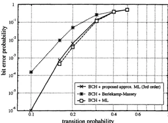
transitionprobability

Figure 4.2: Comparison of decoding

perfor-mances for a BCH code with $k=7$ and $n=63$.

Horizontal axis: transition probability $\epsilon$

.

Verti-cal axis: bit

error

probability. $\cross$: 3rd order

ap-proximateML decoding. $*$: Berlekamp-Massaey

decoding. $\square$: ML decoding.

codes with Berlekamp-Massey decoding for comparison. The results are summarized in Figure

4.1.

Here, the horizontal axis is the code rate $r=k/n$, and the vertical axis is the bit

error

probability. The plots $+$ ($\cross$ resp.) correspond to the 2nd (3rd resp.) order approximate ML

(4.5), and $*$

are

the results on several BCH codes

$(n=7,15,31,63,127,255,511)$

with

Berlekamp-Messey decodings. For the proposed method, we randomly construct a systematic

generator matrix in such a way that each column except for the systematic part has the

same

weight (i.e. number ofnon-zero elements) $w$

.

To be more specific, the submatrix composed by

the first $k$ columns of the generator matrix is set to be an identity matrix in order to make the

code systematic, while the rest of the generator matrix is made up of $k\cross k$ random matrices

generatedbyrandom permutationsofcolumns ofacirculant matrix,whose first column is given

by

$(1, \cdots 1,0, \cdots 0)^{t}\check{w}$

.

The

reason

for using random codings is that

we

want to investigate average behaviors of the

decoding performance, and, for this purpose, we do not put unnecessary additional structure

at encodings. The number of matrices added after the systematic part depends on the code

rate, and the plot for each code rate corresponds to the best result obtained out of about 100

realizations of the generator matrix. Also,

we

have employed $w=3$ and 2 for the generator

matrices of the 3rd and the 2nd order approximate ML, respectively. Moreover, the length of

the codewords $n$

are

assumed to be up to 512. $\mathbb{R}om$ Figure 4.1, we can see that the proposed

method with the 3rd order approximate ML $(\cross)$ achieves better performance than that of BCH

codes with Berlekamp-Massey$(*$$)$. It should be also noticed that the decoding performance

reasonable because of the meaning of

the

Taylor expansion.

Next, let

us

directly compare the decoding performances among ML, approximate ML (3rd

order) and Berlekamp-Massey by applying them

on

the

same

BCH code $(k=7, n=63)$

.

The

result

on

thebit

error

probability withrespect to transitionprobability is shown in Figure4.2.

This figure clearly shows that the performance of the 3rd order approximate ML decoding is far

better than that of Berlekamp-Massey decoding (e.g., improvement ofdouble-digit at $\epsilon=0.1$).

Furthermore, it should be noted that the 3rd order approximate ML decoding achieves

a

very

close bit

error

performance to that of ML decoding. Although

we

have not mathematically

confirmed the computational complexity of the proposed approach, the computational time

of the approximate ML (3rd order) is much faster than ML decoding. This fact about low

computationalcomplexityof the approximate ML is explained

as

follows: Non-zero higher order

terms in (4.6) appear

as

a

result of linear dependent relations of columnvectors of$G$, however,

linear dependences require high

codimentional

scenario. Hence, most of the higher order terms

become

zeros.

As

a

result, the computational complexity for the approximate ML, which is

determined bythe number of

nonzero

terms in the expansion, becomes small.

In conclusion, these numerical simulations suggest that the 3rd order approximate ML

de-coding approximates ML dede-coding very well with low computational complexity. We notice

that the encodings examined here

are

random codings. Hence, we

can

expect to obtain better

bit

error

performance by introducing certain structure

on

encodings suitable to this proposed

decoding rule, or much

more

exhaustive search of random codes. One of the possibility will be

the combination with Theorem 1. Onthe other hand, it is also possible to consider suitable

en-coding rules from the viewpoint ofdynamicalsystemsviarational maps (4.1). Theseimportant

subjects are discussed in Section 5 [1] in detail.

Acknowledgment

The authors express their sincere gratitude to the members of TIN working group for valuable

commentsand discussions

on

thispaper. The authorsalso wish tothankShiro Ikedafor pointing

out

a

relationship of this work to information geometrydiscussed in [2]. This work is supported

by JST PRESTO program.

References

[1] K. Hayashi and Y. Hiraoka, Rational Maps and Maximum Likelihood Decodings,

http: //arxiv.org$/pdf/1006.5688vl$

[2] S. Ikeda, T. Tanaka, and S. Amari, Information Geometry of Turbo and Low-Density

Parity-Check Codes, IEEE Rans. Inform. Theory, vol. 50, pp. 1097-1114,

2004.

[3] C. E. Shannon, A Mathematical Theory ofCommunication, Bell System Technical Journal,