On localized trapped modes in a pipe-cavity system (Mathematical Aspects and Applications of Nonlinear Wave Phenomena)

全文

(1)32. 数理解析研究所講究録第2076巻 2018年 32-42. On localized trapped modes in a pipe‐cavity system Mikael A. Langthjem†, Masami Nakano‡ † Faculty of Engineering, Yamagata University, Jonan 4‐chome, Yonezawa‐shi, 992‐8510 Japan ‡Institute of Fluid Science, Tohoku University, 2‐1‐1 Katahira, Aoba‐ku, Sendai‐shi, 980‐8577 Japan Abstract. The work is concerned with an analytical study of acoustic trapped modes in a cyhndrical expansion chamber, placed in between two semi‐infinite pipes (waveguides). Trapped mode solutions are expressed in terms of Fourier‐Bessel series, with the expansion coefficients determined from a determinant condition. The roots of the determinant, expressed in terms of the wavenumber k , correspond to trapped modes. In the case of a shallow cavity, in the sense that the cavity radius is only slightly larger than the pipe radius, asymptotic approximations for the coeficients of the determinant can be apphed. The determinant then reduces to a simple form with four‐rowed minors placed on a diagonal, enabling analytical evaluation and a proof of existence of trapped modes. We consider here circumferential mode numbers m\geq 1 . For a shallow cavity and for low values of the circumferential mode number there is just one trapped mode in the allowable wave number domain k_{\min}<k<k_{\mathrm{m}\mathrm{w}} , where k_{\min} is the cutoff frequency for acoustic waves in the cavity and k_{\max} is the corresponding cutoff frequency in the pipes. This mode is symmetric about a radial axis in the center of the cavity.. 1. Introduction. The existence of trapped modes in a variety of physical systems has received much attention for more than sixty years and it is now known that trapped modes may be found across a wide range of length scales, from waveguides in the ocean, over acoustic and elastic waveguides, to. quantum waveguides [5]. A trapped mode, also called a localized mode, refers to an infinite medium in a state of linear oscillations only in the vicinity of an object or a geometrical fea‐ ture which can act as a resonator. There is no radiation of energy to infinity; the energy is also trapped, or localized. One reason for the attention these problems have received is math‐ ematical: the trapped modes, characterized by a discrete wavenumber spectrum, co‐exist with the continuous spectrum which is characteristic for guided waves in an infinite domain. The solutions to these problems are thus non‐unique even though the problems are hnear. The present paper gives an analytical solution to the problem of acoustic trapped modes in a cylindrical expansion chamber, placed in between two semi‐infinite pipes, i.e. waveguides, \mathrm{a}. problem which previously has been investigated just numerically [2]. The existence of trapped modes is proved in the case of a shallow cavity, shallow in the sense that the radius of the cavity is only slightly larger than the radius of the connecting pipes..

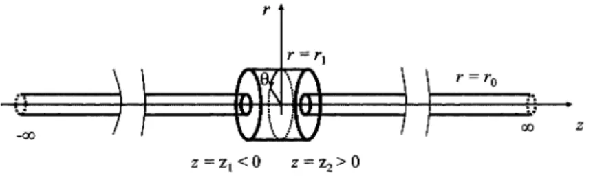
(2) 33. 2. Problem formulation Consider a cylindrical cavity — an expansion chamber — connected with two semi‐infinite. cylindrical pipes (wave guides), as shown in figure 1.. z. z=\mathrm{z}_{1}<0 z=\mathrm{z}_{2}>0. Figure 1: Sketch of the configuration.. Let the radius of the pipes be. r_{0}. and let the radius of the cavity be. cavity L_{1}=z_{2}-z_{1} . Cyhndrical polar coordinates. z, r, $\theta$. r_{1} .. The length of the. will be used. The propagation of sound. through the system is governed by the wave equation. \displayst le\frac{\partial^{2}$\phi$}{\partialt^{2}=c_{0}^{2}\nabl ^{2}$\phi$ ,. (1). \nabla $\phi$\cdot n=0. (2). subject to the Neumann condition. on the sohd boundaries. Here $\phi$(t, z, r, $\theta$) is the velocity potential, with t being the time, c_{0} is the speed of sound, and n is the inward pointing normal vector. The Laplacian in cylindrical polar coordinates is given by. \displayst le\nabla^{2}=\frac{1}r\frac{\partial}{\partialr}(\frac{\partial}{\partialr})+\frac{1}r^{2}\frac{\partial^{2}{\partial$\theta$^{2}+\frac{\partial^{2}{\partialz^{2} .. (3). The sound pressure p(t, z, r, $\theta$) is given by. (4). p=- $\rho$\partial $\phi$/\partial t, where. $\rho$. is the fluid density. The acoustic particle velocity u=(u_{z}, u_{r, $\theta$}u) is given by \mathrm{u}=\nabla $\phi$ .. 3. (5). Construction of a trapped mode We will here consider the construction of a trapped mode. By employing the method of. separation of variables, the solution to (1) can be expressed in the form of a Fourier‐Bessel series. In the cavity domain. z_{1}<z<z_{2}. the mode. m. solution can be written. $\phi$_{1m}=\displaystyle\sum_{n=0}^{\infty}$\phi$_{\mathrm{i}mn}=\sum_{n=0}^{\infty}\{C_{mn}\mathrm{e}^{\mathrm{i}k_{1mn}z +D_{mn}\mathrm{e}^{-\mathrm{i}k_{1mn}z \}J_{m}(j_{mn}\frac{r}{r_{1} ). ,. (6).

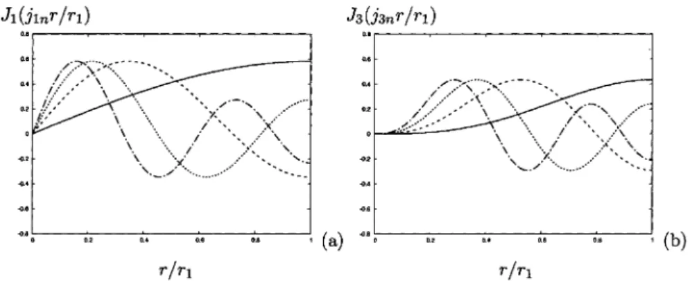
(3) 34. where. m. is the circumferential mode number, C_{mn} and D_{mn} are constants, J_{m}(z) is the Bessel m, j_{mn} are the zeros of J_{m}'(z) , where the dash denotes differen‐. function of first kind and order. tiation with respect to the argument z , and. k_{1mn}^{2}=k^{2}- (\displaystyle \frac{j_{mn} {r_{1} )^{2} k=\frac{ $\omega$}{c_{\mathrm{O}. .. (7). A factor \mathrm{e}^{-\mathrm{i} $\omega$ t}\mathrm{e}^{\mathrm{i}m $\theta$} has been suppressed. The zeros j_{mn} are ordered such that. jm0\leq jm\mathrm{i}\leq jm2\leq.. .. (8). It is noted also that m\leq j_{m0} [ 1 , p. 370]. The complete solution is given by $\phi$_{1}=\displaystyle \sum_{m}$\phi$_{1m} . In the following a single, fixed value of. m. will be considered rather than the sum over. m. . This is. equivalent to the approach in [8]. The function J_{m}(j_{mn}r/r_{1}) , 0 \leq r/r_{1} \leq 1 , is shown in figure 2 for n=0 , 1, 2, and 3, with m=1 in part (a) and with m=3 in part (b). For any value of m the value of n corresponds to the number of nodal points in the domain 0\leq r/r_{1}\leq 1 ; thus there are no nodal point for n=0, one nodal point for n=1 , etc. As part (b) indicates, the larger the value of m the ‘flatter’ are the graphs by small values of r/r_{1}.. J_{1}(j_{1n}r/r_{1}). J_{3}(j_{3n}r/r_{1}). r/r_{1} r/r_{1} Figure 2: The function J_{m}(j_{mn}r/r_{1}) plotted in the range 0\leq r/r_{1} \leq 1 with m=1 in (a) and m=3 in (b). Plain lines: n=0 ; broken hnes: n=1 ; dotted lines: n=2 ; dash‐dot lines: n=3.. In order to construct a trapped mode we consider the following mode. domains. In the left hand domain. -\infty<z<z_{1} ,. m. solutions in the pipe. the left‐going (outgoing) wave. $\phi$_{0m}^{-}=\displaystyle \sum_{n=0}^{\infty}A_{mn}J_{m}(j_{mn}\frac{r}{r_{0} )\mathrm{e}^{-\mathrm{i}k_{0mn}z}, -\infty<z<z_{1}<0. ,. (9). where. and in the right‐hand domain. k_{0mn}^{2}=k^{2}- (\displaystyle \frac{j_{mn} {r_{0} )^{2}. z_{2}<z<\infty ,. (10). the right‐going (and again outgoing) wave. $\phi$_{0m}^{+}=\displaystyle \sum_{n=0}^{\infty}B_{mn}J_{m}(j_{mn}\frac{r}{r_{0} )\mathrm{e}^{\mathrm{i}k_{0mn}z}, 0<z_{2}<z<\infty. .. (11).

(4) 35. The functions k_{0mn} and k_{1mn} in (10) and (7), respectively, are specified as. k_{$\alph$7n}=\left{bgin{ary}l \sqrt{k^2}-(lr_{$\alph$}\mathfrk{B}^\underli {n})^2,k>\frac{j_mn}{r_$\alph$}\ mathr{i}\sqrt(_{$\alph$}^{\mathr{k})^2-{}um,k<\frac{j_mn}{r_$\alph$} \end{ary}\ight.. $\alpha$=0 ,. 1.. (12). It is thus seen that a trapped mode may be present by mode (m, n) if the wavenumber the range. k. \displaystyle \frac{j_{mn} {r_{1} <k<\frac{j_{mn} {r_{0} ,. is in. (13). where j_{mn}/r_{0} is the cutoff frequency for mode (m, n) for a pipe of radius r_{0} and j_{mn}/r_{1} is the cutoff frequency for mode (m, n) for a pipe of radius r_{1} . This is because, with this specification of k , the solution has the form \mathrm{e}^{\pm \mathrm{i}|k_{1mn}z|} in the cavity domain and the form \mathrm{e}^{-|k_{0mn}z|} in the pipe domains.. It is noted that the expansions (6), (9), (11) constitute complete sets of functions [7]. These functions must satisfy matching and boundary conditions at the steps. At are given by. z=z_{1}. these conditions. $\phi$_{m0}^{-}(z_{1-}) = $\phi$_{1m}(z_{1+}) , 0<r<r_{0} ,. (14). \displaystyle \frac{\partial$\phi$_{0m}^{-} {\partial z}(z_{1-}) = \frac{\partial$\phi$_{1m} {\partial z}(z_{1+}) , 0<r<r_{0} , \displaystyle \frac{\partial$\phi$_{1m}}{\partial z}(z_{1+}) = 0, r_{0}<r<r_{1} . Similar conditions apply at. \displaystyle\frac{\partial$\phi$_{0m}{\partialr}|_{r= 0}=0. z=z_{2} .. for. (15) (16). It is noted that the boundary conditions. z_{1}<z<z_{2},. \displaystyle\frac{\partial$\phi$_{1m}{\partialr}|_{r= _{1}=0. for. z<z_{1}, z>z_{2} ,. (17). which apply as well, are exactly satisfied by the solutions (6), (9), and (11). The conditions (14) (at z=z_{1}, z_{2} ) are Dirichlet conditions, while (15) and (16) (also at z=z_{1}, z_{2} ) are Neumann conditions.. The mixed boundary value problem (6), (9), (11) and (14) -(16) (again with similar conditions z_{2} ) can be discretized by converting the boundary conditions (14)‐(16) to a applying at z =. Galerkin weak formulation, using the weight functions residual equations take the forms. J_{m}(j_{mq}\displaystyle \frac{r}{r0})r and J_{m}(j_{mq}\displaystyle \frac{r}{r_{1} )r .. \displaystyle \int_{0}^{r_{0} \{$\phi$_{0m}(z_{1-})-$\phi$_{1m}(z_{1+})\}J_{m}(j_{mq}\frac{\prime r}{r_{0} ) rdr=0 , \displaystyle \int_{0}^{r_{0} \{\frac{\partial$\phi$_{0m} {\partial z}(z_{1-})-\frac{\partial$\phi$_{1m} {\partial z}(z_{1+})\}J_{m}(j_{mq}\frac{r}{r_{1} ) rdr=0 ,. The. (18). (19). and. \displaystyle \int_{r0}^{r_{1} \frac{\partial$\phi$_{1m} {\partial z}(z_{1+})J_{m}(j_{mq}\frac{r}{r_{1} ) rdr=0 , for q=0 , 1, 2,. \cdots. (20). . Combining (19) with (20) we get. \displaystyle \int_{0}^{r_{0} \frac{\partial$\phi$_{0m} {\partial z}\partial z(z_{1-})J_{m}(j_{m\mathrm{q} \frac{r}{r_{1} )rdr-\int_{0}^{r_{1} \frac{\partial$\phi$_{1m} {\partial z}(z_{1+})J_{m}(j_{mq}\frac{r}{r_{1} ) rdr=0 .. (21).

(5) 36. 4. Nondimensionalization Next we make the equations nondimensional by introducing the nondimensional parameters. \displaystyle \tilde{r}=\frac{r}{r_{0} , \hat{r}=\frac{r}{r_{1} , \tilde{z}=\frac{z}{r_{0} , \tilde{k}=kr_{0}, $\alpha$=\frac{r_{0} {r_{1} .. (22). \tilde{k}_{0mn}=\mathrm{i}\sqrt{j_{mn}^{2}-\tilde{k} , \tilde{k}_{1mn}=\sqrt{\tilde{k}-$\alpha$^{2}j_{mn}^{2} .. (23). Also, let. The three series solutions (6), (9), and (11) are now expressed in the forms. $\phi$_{\mathrm{i}m=\displaystyle\sum_{n=0}^{\infty}\{C_{mn}\mathrm{e}^{\mathrm{i}\tilde{k}_{1mn}(\tilde{z}-\tilde{z}_{1})+D_{mn}\mathrm{e}^{-\mathrm{i}\tilde{k}_{1mn}(\tilde{z}-\overline{z}_{2})\} frac{1}{\tilde{k}_{1mn}\frac{J_{m}(j_{mn}$\alpha$\tilde{r}){J_{m}^{2}(j_{mn})\frac{2j_{mn}^{2}{j_mn}^{2}-m^{2}. $\phi$_{0m}^{-}=\displaystyle\sum_{n=0}^{\infty}A_{mn}\mathrm{e}_{J_{m}^{2}(j_{mn})j_{mn}^{2}^{-\mathrm{i}\tilde{k}_{0mn}(1}\overline{z}-\overline{z})^{J_{m}(j_{mn}\tilde{r})2j_{mn}^{2}. \overline{-m^{2}}. ’. -\infty<\overline{z}<\tilde{z}_{1} <0,. ,. (24). (25). and. $\phi$_{0m}^{+}=\displaystyle\sum_{n=0}^{\infty}B_{mn}\mathrm{e}^{\mathrm{i}\tilde{k}_{0mn}(\tilde{z}-\tilde{z}_{2}) \frac{J_{m}(j_{mn}\tilde{r}) {J_{m}^{2}(j_{mn}) \frac{2j_{mn}^{2} {j_{mn}^{2}-m^{2} ,0<\tilde{z}_{2}<\tilde{z}<\infty 5. .. (26). Determinant condition. The matching and boundary conditions (18) and (21), evaluated at \overline{z}=\tilde{z}_{1} and \tilde{z}=\tilde{z}_{2} , can with (24), (25), and (26) inserted be written. \displaystyle\sum_{n=0}^{\infty}\{$\delta$_{qn}A_{mn}-\mathcal{F}_{1mqn}C_{mn}-\mathcal{F}_{1mqn}\mathrm{e}^{\mathrm{i}\overline{k}_{1mn}(\overline{z}_{2}-\tilde{z}_{1}) D_{mn}\ =0 \displaystyle\sum_{n=0}^{\infty}\{$\delta$_{qn}B_{mn}-\mathcal{F}_{1mqn}\mathrm{e}^{\mathrm{i}\tilde{k}_{1mn}(\tilde{z}2-\overline{z}_{1}) C_{mn}-\mathcal{F}_{1mqn}D_{mn}\ =0, \displaystyle\sum_{n=0}^{\infty}\{ overline{f}_{2mqn}A_{mn}+$\delta$_{qn}C_{mn}-$\delta$_{qn}\mathrm{e}^{\mathrm{i}\overline{k}_{1mn}(\tilde{z}_{2}-\overline{z}_{1}) D_{mn}\ =0, \displaystyle \sum_{n=0}^{\infty}\{21, ,. for q=0 , 1,. \cdots. (27). , where $\delta$_{\mathrm{q}n} is Kronecker’s delta and. \displaystyle\mathcal{F}_{1mqn}=\frac{2$\alpha$^{2}j_{mn}^{2} {j_{mn}^{2}-m^{2} $\alpha$^{2}j_{mn}^{2}-j_{mq}^{2}\tilde{k}_{1mn}^{-1}\frac{1}{J_{m}^{2}(j_{mn}). (28). \displaystyle\mathcal{F}_{2mqn}=\frac{2$\alpha$^{2}j_{mn}^{2} {j_{mn}^{2}-m^{2} j_{mn^{-$\alpha$^{2}j_{mq}^{2} ^{2^{\tilde{k}_{0mn} \frac{1}{J_{m}^{2}(j_{mn}). (29). \times\{ $\alpha$ j_{mn}J_{m+1}($\alpha$_{jmn})J_{m}(jmq)-J_{m}( $\alpha$ jmn)J_{m+1(jmq})\},. \times\{j_{mn}J_{m+1(jmn})J_{m}( $\alpha$ jmq)- $\alpha$ J_{m}(jmn)J_{m+1}( $\alpha$ j_{mq})\}..

(6) 37. The fUmctions (28) and (29) have been obtained by employing the relations [9, Ch. V]. \displaystyle \int_{0}^{1}J_{m}(j_{mn}\tilde{r})J_{m}(j_{m\mathrm{q} \tilde{r})\tilde{r}d\overline{r}=\frac{1}{2}\frac{$\delta$_{qn} {j_{mq}^{2} [j_{mn}^{2}-m^{2}]\{J_{m}(j_{mn})\}^{2}. ,. (30). and. \displaystyle \int_{0}^{1}J_{m}(j_{mn} $\alpha$\hat{r})J_{m}(j_{mq}\hat{r})\hat{r}d\hat{r}=\frac{1}{j_{mn}^{2}-j_{m\mathrm{q} ^{2}. (31). \times\{-\}.. Written in matrix form, (27) can be expressed as Ab where \mathrm{b}. =. denoted by. =\mathrm{O} ,. \{A_{m0}B_{m0}C_{m0}D_{m0}A_{m1}B_{m1}C_{m1}D_{m1} . . . \}^{T} . a_{qn}, q, n=0 ,. value of the wavenumber. (32) The elements of the matrix A are. 1, . The condition for the existence of a trapped mode at a given \tilde{k} is that the infinite determinant \cdots. \triangle=\det \mathrm{A}=|a_{qn}|_{0}^{\infty}=0 .. (33). In terms of the nondimensional variables a trapped mode may exist in mode (m, n) in the wavenumber range. $\alpha$ j_{mn}<\tilde{k}<j_{mn} .. 6. (34). Symmetric and antisymmetric solutions. It is seen directly from (27) that two types of solutions are possible: symmetric solutions, $\phi$(z) = $\phi$(-z) , and antisymmetric solutions, $\phi$(z) =- $\phi$(-z) . By symmetric solutions, A_{mn}= B_{mn} , and C_{mn}=D_{mn} , for any -D_{mn} , for any. m,. n. m,. n. . By antisymmetric solutions, A_{mn}= -B_{mn} , and C_{mn}=. . In both cases, (27) reduces to the following system of just two equations:. \displaystyle\sum_{n=0}^{\infty}\{$\delta$_{qn}A_{mn}-\mathcal{F}_{1mqn}C_{mn}(1\pm\mathrm{e}^{\mathrm{i}\overline{k}_{1mn}(\tilde{z} 21 \displaystyle\sum_{n=0}^{\infty}\{ mathcal{F}_{2mqn}A_{mn}+$\delta$_{qn}C_{mn}(1\mp\mathrm{e}^{\mathrm{i}\overline{k}_{1mn}(\tilde{z}_{2}-\tilde{z}_{1}) \}=0,. ,. q=0 , 1,. \cdots. (35). . In each of these two equations the upper sign (before the exponential function). gives the symmetric solution, while the lower sign gives the antisymmetric solution.. 7. The case of a shallow cavity Here we consider the case where $\alpha$\approx< 1 , that is to say,. $\alpha$. is shghtly smaller than one. Use. will be made of the expansion [1, p. 363]. J_{m}( $\alpha$\displaystyle \tilde{r}j_{mn})=$\alpha$^{m}\sum_{p=0}^{\infty}\frac{1}{p!}(-1)^{p}($\alpha$^{2}-1)^{p}J_{m+p}(\tilde{r}j_{mn}). .. (36).

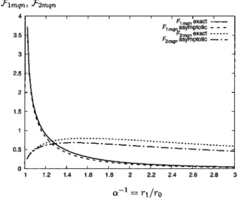
(7) 38. Let $\epsilon$=1- $\alpha$ . For 0< $\epsilon$\ll 1 we can write. J_{m}( $\alpha$\tilde{r}j_{mn})=$\alpha$^{m}J_{m}(\overline{r}j_{mn})+O( $\epsilon$) .. (37). The functions \mathcal{F}_{1mqn} and \mathcal{F}_{2mqn} , defined by (28) and (29), then reduce to. \mathcal{F}_{1mqn}\approx$\delta$_{qn}$\alpha$^{m+2}\tilde{k}_{1mn}^{-1}, \overline{J^{-} _{2mqn}\approx$\delta$_{\mathrm{q}n}$\alpha$^{m}\tilde{k}_{0mn} .. (38). A comparison between the‘full’ functions \mathcal{F}_{1mqn} and \overline{J^{-} _{2mqn} and their asymptotic approximations n 0 , and with \overline{k} 1, q (38) is shown in figure 3. The graphs are obtained with m =. \displaystyle \frac{1}{2}j_{10}( $\alpha$+1) . when n. =. =. =. As would be expected, the agreements are very good when $\alpha$ is close to one, i.e. is small, and less good otherwise. The trends are similar for any values of m, q,. $\epsilon$=1- $\alpha$. , and \tilde{k}.. \mathcal{F}_{1mqn}, \mathcal{F}_{2mqn} 3. 2. 1. 0. $\alpha$^{-1}=r_{1}/r_{0} Figure 3: Comparisons between the functions \overline{f^{\sim} _{1mqn} and \overline{f}_{2mqn} , defined by (28) and (29), and their asymptotic approximations, defined by (38). Employing (38) the system (27) reduces to. \displaystyle\sum_{n=0}^{\infty}$\delta$_{qn}\{A_{mn}-\frac{$\alpha$^{m+2}{\tilde{k}_{1mn}C_{mn}-\frac{$\alpha$^{m+2}{\tilde{k}_{1mn}\mathrm{e}^{\mathrm{i}\tilde{k}_{1mn}()\tilde{z}2-\overline{z}1D_{mn}\=0 \displaystyle\sum_{n=0}^{\infty}$\delta$_{qn}\{B_{mn}-\frac{$\alpha$^{m+2}{\tilde{k}_{1mn}\mathrm{e}^{\mathrm{i}\tilde{k}_{1mn}()\overline{z}_{2-\tilde{Z}1C_{mn}-\frac{$\alpha$^{m+2}{\tilde{k}_{1mn}D_{mn}\=0, \displaystyle\sum_{n=0}^{\infty}$\delta$_{qn}\{$\alpha$^{m}\overline{k}_{0mn}A_{mn}+C_{mn}-\mathrm{e}^{\mathrm{i}\tilde{k}_{1mn}(\tilde{z}2-\tilde{z}_{1}) D_{mn}\ =0, \displaystyle\sum_{n=0}^{\infty}$\delta$_{qn}\{$\alpha$^{m}\overline{k}_{0mn}B_{mn}-\mathrm{e}^{\mathrm{i}\tilde{k}_{1mn}(\tilde{z}_{2}-\tilde{z}_{1}) C_{mn}+D_{mn}\ =0, ,. q=0 ,. (39). 1, . That is to say, the determinant decouples into four‐rowed minors [4, p. 20], i.e., blocks of size 4\times 4 , placed on a diagonal, and with zeros elsewhere. The (determinant of the) \cdots.

(8) 39. minor no.. n. is evaluated as. $\Delta$_{n}=2\displaystyle\frac{\mathrm{e}^{\mathrm{i}\overline{k}_{1mn}(\tilde{z}-\tilde{z}_{1})2}{\tilde{k}_{1mn}[2\tilde{k}_{0mn}\overline{k}_{1mn}$\alpha$^{2(m+1)}\cos(\overline{k}_{1mn}(\tilde{z}_{2}-\overline{z}_{1}). (40). -\mathrm{i}(\overline{k}_{0mn}^{2}$\alpha$^{4(m+1)}+\tilde{k}_{1mn}^{2})\sin(\tilde{k}_{1mn}(\tilde{z}_{2}-\tilde{z}_{1}) ].. The original determinant is evaluated as $\Delta$=\displaystyle \prod_{n=0}^{\infty}\triangle_{n}. Consider first the case where \tilde{k}_{\approx}> $\alpha$ j_{mn} ( \tilde{k} is just slightly larger than $\alpha$ j_{mn} ), specifically let $\delta$^{2}=\overline{k}^{2}-$\alpha$^{2}j_{mn}^{2}, 0<$\delta$^{2}\ll 1 . Then \tilde{k}_{1mn}= $\delta$ and \tilde{k}_{0mn}\approx \mathrm{i}j_{mn}(1-$\alpha$^{2})^{\frac{1}{2} . Inserting this into. (40) gives. \displaystyle\frac{1}{2}\frac{\tilde{k}_{1mn}{\mathrm{e}^{\mathrm{i}\tilde{k}_{1mn}(\overline{z}_{2}-\overline{z}_{1}) \triangle_{n}\ap rox\mathrm{i}[\mathrm{S}. (41). -(-j_{mn}^{2}$\alpha$^{4(m+1)}(1-$\alpha$^{2})+$\delta$^{2})\sin( $\delta$(\tilde{z}_{2}-\tilde{z}_{1}) ] \approx \mathrm{i} $\delta$[2j_{mn}(1-$\alpha$^{2})^{\frac{1}{2} $\alpha$^{2(m+1)}+j_{mn}^{2}$\alpha$^{4(m+1)}(1-$\alpha$^{2})(\overline{z}_{2}-\tilde{z}_{1})].. Consider next the case where \overline{k} \ap rox< j_{mn} ( \tilde{k} is just slightly smaller than j_{mn} ), specifically let 0<$\delta$^{2}\ll 1 . Then \tilde{k}_{0mn}=\mathrm{i} $\delta$ and \tilde{k}_{1mn}\approx j_{mn}(1-$\alpha$^{2})^{\frac{1}{2} . Inserting this into (40). $\delta$^{2}=j_{mn}^{2}-\overline{k}^{2}, gives. \displaystyle\frac{1}{2}\frac{\tilde{k}_{1mn} {\mathrm{e}^{\mathrm{i}\tilde{k}_{1mn}(\tilde{z}_{2}-\tilde{z}1 )}$\Delta$_{n}\ap rox\mathrm{i}[2$\delta$j_{mn}(1-$\alpha$^{2})^{\frac{1}{2} $\alpha$^{2(m+1)}\cos(j_{mn}\sqrt{1-$\alpha$^{2} (\tilde{z}_{2}-\tilde{z}_{1}). (42). -(-$\delta$^{2}$\alpha$^{4(m+1)}+j_{mn}^{2}(1-$\alpha$^{2}) \sin(j_{mn}\sqrt{1-$\alpha$^{2} (\tilde{z}_{2}-\tilde{z}_{1}) ] \approx \mathrm{i}[2 $\delta$ j_{mn}(1-$\alpha$^{2})^{\frac{1}{2} $\alpha$^{2(m+1)} -(-$\delta$^{2}$\alpha$^{4(m+1)}+j_{mn}^{2}(1-$\alpha$^{2}) (j_{mn}\sqrt{1-$\alpha$^{2} (\tilde{z}_{2}-\tilde{z}_{1})]. \approx -\mathrm{i}j_{mn}^{3}(1-$\alpha$^{2})^{\frac{3}{2} (\overline{z}_{2}-\tilde{z}_{1}). .. -\displaystyle\mathrm{i}^{\tilde{k} \frac{1}{2}\ovalbox{\t \smal REJECT}_{2}\triangle_{n}\mathrm{e}^{1} is real and >0 for \overline{k}_{\approx}> $\alpha$ j_{mn} , while in the second case, (42) shows that -\displayst le\mathrm{i}^ \overline{k} \frac{1} 2 \ovalbox{\t smal REJ CT}_{1}\triangle_{n}\mathrm{e}^{\mathrm{i}k_{1mn}(\overline{z}_{2}-\overline{z}) is real and <0 for \tilde{k}_{\approx}<j_{mn} . It is noted, In the first case, (41) clearly shows that. also, that neither \mathrm{e}^{\mathrm{i}\tilde{k}_{1mn}(\tilde{z}2-\overline{z}_{1})} nor \tilde{k}_{1mn} is zero in $\alpha$ j_{mn}<\tilde{k}<j_{mn} . Thus \triangle_{n} (and thus. \triangle ). has,. at least, one zero for $\alpha$ j_{mn}<\tilde{k}<j_{mn} . To locate one or more of these zeros, set \triangle_{n}=0 and let \tilde{k}=\tilde{s}j_{mn} . Using (40), the expression for \triangle_{n}=0 can be written as. \displaystyle\mathrm{t}\mathrm{m}( \tilde{z}_{2}-\tilde{z}_{1})j_{mn}(\tilde{s}^{2}-$\alpha$^{2})^{\frac{1}{2})=$\alpha$^{2(m+1)}\frac{(1-\tilde{s}^{2})^{\frac{1}{2}(\tilde{s}^{2}-$\alpha$^{2})^{\frac{1}{2} {$\alpha$^{4(m+1)}(\tilde{s}^{2}-1)+(\tilde{s}^{2}-$\alpha$^{2}) Assuming that \tilde{s}\approx $\alpha$<1\approx we can use that \tan(\cdots)\approx(\cdots) . Using also that (43) gives that. or equivalently. .. (43). (1-\displaystyle \tilde{s}^{2})^{\frac{1}{2} \approx 1-\frac{1}{2}\tilde{s},. \displayst le\tilde{s}=\{ frac{$\alpha$^{2(m+1)}+(\tilde{z}_2}-\tilde{z}_1})j_{mn}($\alpha$^{2}+$\alpha$^{4(m+1)} {\frac{1}2$\alpha$^{2(m+1)}+(\tilde{z}_2}-\tilde{z}_1})j_{mn}(1+\grave{$\alpha$}^{4(m+1)} \^{\frac{1}2. (44). \displaystyle\tilde{s}^{2}=1+\frac{\frac{1}2$\alpha$^{2(m+1)}-(\tilde{z}_{2}-\tilde{z}_{1})j_{mn}(1-$\alpha$^{2}){\frac{1}2$\alpha$^{2(m+1)}+(\tilde{z}_{2}-\tilde{z}_{1})j_{mn}(1+$\alpha$^{4(m+1)}. (45). .. In order to satisfy the condition $\alpha$ j_{mn} < \overline{k} <j_{mn} it is necessary that $\alpha$ <\tilde{s}< 1 . It is clearly possible to choose a cavity length \tilde{z}_{2}-\tilde{z}_{1} such that this condition is satisfied. In particular,.

(9) 40. \tilde{s}< 1 if \tilde{z}_{2}-\tilde{z}_{1} >$\alpha$^{2(m+1)}/\{(1-$\alpha$^{2})j_{mn}\} . (It is noted that the lowest possible value of j_{mn} is j_{10}=1.8412\cdots.) We finaly discuss the limit $\alpha$\rightarrow 1 , where the cavity disappears altogether. In this hmit (13) degenerates into a single point, \tilde{k}=j_{mn} . Then, from (23) we obtain \tilde{k}_{0mn} =\tilde{k}_{1mn} =0 . Thus. there is no wave motion and no meaningful solution to the problem, as there shouldn’t be either. In the following we check (45) in this limit. As $\alpha$ \rightarrow 1, \tilde{k} \rightarrow \overline{k}_{\max} , that is, \tilde{k} \rightarrow j_{mn} , the. cutoff frequency of the pipes. This means that root function. (1-\tilde{s}^{2})^{\frac{1}{2}. \tilde{s}\rightarrow 1. in (43). Then, in (44) and (45), the square. needs to be approximated not for. \tilde{s}. small but for 1-\tilde{s}^{2} small. Here use. can be made of Lanczos’s power expansion of y=\sqrt{x} in terms of Chebyshev polynomials [3, \mathrm{p}. 485]. The first approximation is simply y_{1} =x . Using this approximation in (43), (45) takes the form. \displaystyle\overline{s}^{2}\ap rox1-\frac{(\tilde{z}_{2}-\tilde{z}_{1})j_{mn}(1-$\alpha$^{2}) {$\alpha$^{2(m+1)}+(\tilde{z}_{2}-\tilde{z}_{1})j_{mn}(1+$\alpha$^{4(m+1)} which correctly gives that. 8. \tilde{s}\rightarrow 1 ,. and thus that \tilde{k}\rightarrow\overline{k}_{\max}=j_{mn} , as. ,. (46). $\alpha$\rightarrow 1.. Symmetric and antisymmetric solutions in the case of a shal‐ low cavity Employing the shallow cavity approximation (38) to the two equations (35), they reduce to. \displaystyle\sum_{n=0}^{\infty}$\delta$_{qn}\{A_{\mathfrak{m}n-\frac{$\alpha$^{m+2}{\tilde{k}_{1mn}C_{mn}(1\pm\mathrm{e}^{\mathrm{i}\overline{k}_{1mn}(\overline{z}2-\overline{z}_{1}) \}=0 \displaystyle\sum_{n=0}^{\infty}$\delta$_{\mathrm{q}n \{$\alpha$^{m}k_{0mn}A_{mn}+C_{mn}(1\mp\mathrm{e}^{\mathrm{i}\overline{k}_{1mn}(\tilde{z} 2-\tilde{z}_{1}) \}=0. ,. (47). Here the upper signs correspond to the solution \mathrm{s}\mathrm{y}\mathrm{n}$\alpha$\mathrm{n}\mathrm{e}\mathrm{t}\mathrm{r}\mathrm{i}\mathrm{C}_{\backsla h} about the r axis, while the lower signs correspond to the antisynnnetric solution. The determinant of the nth minor is. $\Delta$_{n}=1\displaystyle\mp\mathrm{e}^{\mathrm{i}\tilde{k}_{1mn}(\overline{z}_{2}-\overline{z}_{1})+$\alpha$^{2(m+1)}\frac{\tilde{k}_{0mn}{\tilde{k}_{1mn}(1\pm\mathrm{e}^{\mathrm{i}\tilde{k}_{1mn}(\tilde{z}_{2}-\tilde{z}_{1}). .. (48). We consider first the symmetric case, that is, the upper signs in (48). With these signs (4S) can be written as. $\Delta$_{n}= 2\mathrm{e}^{\mathrm{i}\frac{1}{2}\tilde{k}_{1mn}(\overline{z}_{2}-\tilde{z}_{1})} \times. (49). { $\alpha$^{2(m+1)}\displaystyle\frac{\tilde{k}_{0mn}{\overline{k}_{1mn}\cos(\frac{1}{2}\tilde{k}_{1mn}(\overline{z}_{2}-\overline{z}_{1}) sin (\displaystyle\frac{1}{2}\tilde{k}_{1mn}(\tilde{z}_{2}-\tilde{z}_{1}) }. -\mathrm{i}. Consider first the case where \tilde{k} \ap rox> $\alpha$ j_{mn} ( \tilde{k} is just slightly larger than $\alpha$ j_{mn} ), as done in the previous section. Then. \tilde{k}_{1mn}. =. $\delta$. and. \tilde{k}_{0mn} \approx \mathrm{i}j_{mn}(1-$\alpha$^{2})^{\frac{1}{2} . Inserting these approximations. into (49) it can be written. \displaystyle \triangle_{n}\ap rox 2$\alpha$^{2(m+1)}j_{mn}\sqrt{1-$\alpha$^{2} \{-\frac{1}{2}(\tilde{z}_{2}-\tilde{z}_{1})+\mathrm{i}$\delta$^{-1}\} .. (50). Consider next the case where \overline{k}_{\approx}<j_{mn} ( \tilde{k} is just slightly smaller than j_{mn} ). Then \overline{k}_{0mn}=\mathrm{i} $\delta$ and \tilde{k}_{1mn}\approx j_{mn}(1-$\alpha$^{2})^{\frac{1}{2} . Inserting these expressions into (49) gives. \displaystyle \triangle_{n}\ap rox\frac{1}{2}j_{mn}^{2}(1-$\alpha$^{2})(\tilde{z}_{2}-\tilde{z}_{1})^{2}-\mathrm{i}j_{mn}\sqrt{1-$\alpha$^{2} (\tilde{z}_{2}-\tilde{z}_{1}) .. (51).

(10) 41. Thus both the real part and the imaginary part change signs. This shows that a symmetric trapped mode exists in the domain. $\alpha$ j_{mn}<\tilde{k}<j_{mn}.. Consider next the antisymmetric case, that is, the lower signs in (48). Then (48) can be written. \triangle_{n} = 2\mathrm{e}^{\mathrm{i}\frac{1}{2}\tilde{k}_{1mn}(\overline{z}-\tilde{z}_{1})}2 \times. (52). { \displaystyle\cos(\frac{1}{2}\tilde{k}_{1mn}(\tilde{z}_{2}-\overline{z}_{1}) -\displayst le\mathrm{i}$\alpha$^{2(m+1)}\frac{\tilde{k}_{0mn}{\tilde{k}_{1mn} sin (\displaystyle\frac{1}{2}\tilde{k}_{1mn}(\overline{z}_{2}-\overline{z}_{1}) }.. In the case where \tilde{k}_{\approx}> $\alpha$ j_{mn} (52) can be approximated as. \triangle_{n}\approx 2+$\alpha$^{2(m+1)}j_{mn}\sqrt{1-$\alpha$^{2} (\tilde{z}_{2}-\overline{z}_{1})+\mathrm{i}O( $\delta$) . In the case where. \tilde{k}<\approx jmn. (53). we get. \triangle_{n}\approx 2+\mathrm{i}j_{mn}\sqrt{1-$\alpha$^{2} (\tilde{z}_{2}-\tilde{z}_{1}) .. (54). The positive real parts in both (53) and (54) indicate that there is no antisymmetric trapped mode in the case of a shallow cavity.. 9. Conclusion In this paper we have carried out an analytical study of acoustic trapped modes in a cyhn‐. drical expansion chamber, connected with two semi‐infinite pipes that are waveguides. The problem has been solved by employing the method of separation of variables, giving Fourier‐. Bessel expansion‐type of solutions in each of the three subregions left pipe, expansion chamber, and right pipe. The solutions for each of these three regions have been hnked via boundary‐ and matching‐conditions, giving an infinite determinant for which the roots correspond to trapped modes. For the case of a shallow cavity—i.e. the cavity radius is only slightly larger than the pipe radius—it has been found that the infinite determinant decouples into four‐rowed minors. (sub‐determinants of dimension. 4\times 4 ). placed along a diagonal, enabling analytical evaluation. into a simple expression. Asymptotic results predicting the existence of trapped modes have been given in this hmit for which there, with low values of the circumferential mode number m, is just one trapped mode in the allowable wave number domain, k_{\min}<k<k_{\max} . It is shown that this mode is symmetric about a radial axis in the center of the cavity. While we have restricted the analytical studies of the present paper to the case of a shallow. cavity, there is mother interesting hmit case that may be studied analytically, namely that of. a narrow cavity ( \overline{z}_{2}-\tilde{z}_{1} small). It may be suspected that a deep, narrow cavity will, in effect, approach a three‐dimensional Helmholtz resonator, that is, a three‐dimensional version of the. first problem studied in [6]. This may be of interest to examine in future work. Acknowledgements We wish to thank Professor Nobumasa Sugimoto of Kansai University for suggesting to us the problem studied. The financial support by Institute of Fluid Science, Tohoku University,. via a ‘Collaborative Research Project 2016‐17 (project codes J16073 and acknowledged.. \mathrm{J}17\mathrm{I}030 ). is gratefully.

(11) 42. References. [1] M. Abramowitz and I. A. Stegun. Handbook of Mathematical Functions. Dover Publications, New York, 1965.. [2] S. Hein and W. Koch. Acoustic resonances and trapped modes in pipes and tunnels. J. Fluid Mech., 605:401−428, 2008.. [3] C. Lanczos. Applied Analysis. Dover Publications, New York, 1988.. [4] L. Mirsky. An Introduction to Linear Algebra. Dover Publications, New York, 1990.. [5] J. Postnova and R. V. Craster. Trapped modes in elastic plates, ocean and quantum waveg‐ Uides. Wave Motion, 45:565−579, 2008.. [6] N. Sugimoto and H. Imahori. Localized mode of sound in a waveguide with Helmholtz resonators. J. Fluid Mech., 546:89−111, 2005.. [7] G. P. Tolstov. Fourier Senes. Dover Publications, New York, 1976. [8]. $\Gamma$ .. Ursel. Trapped modes in a circular cylindrical acoustic waveguide. Proc. R. Soc. Lond.. A, 435:575−589, 1991.. [9] G. N. Watson. Theory of Bessel Functions. Cambridge University Press, Cambridge, 1944..

(12)