An introduction to stochastic processed associated with resistance forms and their scaling limits (Probability Symposium)

An introduction

to

stochastic

_processes

associated

with

resistance

forms

and their

_scaling

limits

D. A.

_Croydon

*

February

3,

2017

Abstract

Weintroduce andsummariseresults from therecent paper‘Scalinglimits of stochasticprocesses

associated withresistanceforms’

_[5],

and alsoapplicationsfrom‘Time‐changesofstochasticprocesses

associated with resistance forms’

_[9],

whichwaswritten_jointlywithT._Kumagai

_{(Kyoto University)}

andB. M._Hambly

_(University

of

_Oxford).

1

Introduction

Theconnectionsbetween

electricity

and

_probability

are

deep,

and have

provided

_manytools for under‐

standing

the behaviour of stochasticprocesses. In thisnote,wedescribea newresultinthis direction from

[5],

which statesthatifa_sequenceof_spaces

_equipped

with so‐called ‘resistance metrics’ andmeasures

convergewithrespecttothe

_{Gromov‐Hausdorff‐vague topology,}

then the associated stochasticprocesses

also _converge.

_(In

thenon‐compactcase,the

proof

in

[5]

alsorequires a

non‐explosion

condition.)

All the relevant concepts will be introduced more

carefully below,

with the statement of the main result

appearingasTheorem 4.1.

This result

_{generalises previous}

workon_trees,

fractals,

andvariousmodels of random

_graphs

_(apart

fromthe

_background

in

_[5],

seealso

_[2,

14

_Moreover,

it isusefulinthe

_study

of

_{time‐changed}

processes,

including

Liouville Brownian_motion, the Bouchaud_trapmodel and the random conductance

_model,

on

suchspaces

[9].

Some of these

examples

will be sketchedinSection 5. Ifurther

conjecture

that the result

will be

applicable

tothe random walkontheincipientinfinite clusterof criticalbond

percolation

onthe

high‐dimensional

integerlattice

_(see

Section

_5.2).

2

Random

walks

on

graphs

and

electrical networks

Before

introducing

the definition ofa resistance metric and associated stochasticprocesson a

general

space,it is

helpful

torecall themore

elementary

definition of effectiveresistanceand the

_{corresponding}

randomwalkon a

_graph.

Thisisthepurposeof thepresentsection.

Westartwith the definition ofarandom walkon a

_{weighted graph.}

In

particular,

let

_{G=(V, E)}

bea

finite,

connected

_{graph, equipped}

with

_(strictly

_positive,

_symmetric)

_edge

conductances

_{(c(x, y))_{\{x,y\}\in E}.}

Let $\mu$beafinitemeasureon Vof

full‐support.

We then define the associated random walkX tobe the

continuous timeMarkov chain withgenerator\triangle,asdefined

by:

( $\Delta$ f)(x):=\displaystyle \frac{1}{ $\mu$(\{x\})}\sum_{y:y\sim x}c(x, y)(f(y)-f(x))

, *

where thesumisoververticesyconnectedtox

by

an

edge

inE, i.e. thisistheprocessthatjumpsfrom

x _{to y}withrate

_{c(x, y)/ $\mu$(\{x\})}

. Notethatthe transitionprobabilitiesof thejumpchainof X aregiven

by

P(x, y)=\displaystyle \frac{c(x,y)}{c(x)},

where

_c(x)

_{:=\displaystyle \sum_{y:y\sim x}c(x, y)}

, andso are

completely

determined

by

the conductances. Themeasure $\mu$

determines the

time‐scaling

of the process. Common choices areto take

_{$\mu$(\{x\}) :=c(x)}

, whichisthe

so‐called constant

speed

random walk

_(CSRW),

or

$\mu$(\{x\}):=1

,whichis the the variable

speed

random

walk

_(VSRW).

As illustrated

_by

the

example presented

inSection_5.4,the lattertwo processescanhave

quitedifferent behaviourifthe conductancesare

_{inhomogeneous.}

Suppose

now we view G as an electrical network with

_{edges assigned}

conductances

_according

to

(c(x, y))_{\{x,y\}\in E}

. If vertices in the network are held

according

to the

potential

f(x)

, then the total

electricalenergy

dissipated

inthenetwork is

given

by

\mathcal{E}(f, f)

,where\mathcal{E} isthe

quadratic

formonV

given

by

\displaystyle \mathcal{E}(f, g):=\frac{1}{2}\sum_{x,y:x\sim y}c(x, y)(f(x)-f(y))(g(x)-g(y))

.

Moreover, regardless

of the

particular

choice of $\mu$,\mathcal{E}isaDirichlet

form

on

L^{2}(V, $\mu$)

, andcanbewritten

as

\displaystyle \mathcal{E}(f, g)=-\sum_{x\in V}( $\Delta$ f)(x)g(x) $\mu$(\{x\})

.

Using

the classical

correspondence

between Dirichlet forms and reversible Markov processes, itfollows

that there is aone‐to‐one

correspondence

between the electricalenergy \mathcal{E}

(viewed

as aDirichlet form

on

L^{2}(V, $\mu$))

and the random walk X.

(For

the definition ofaDirichlet

form,

and

background

onthe

connectionsbetween such

objects

and Markovprocesses,see

[10].)

Suppose

nowthatwewishedto

_replace

ournetwork

_by

a

_single

resistorbetweentwoverticesxand_y.

The resistanceweshouldassignto thisresistortoensurethat thesameamountofcurrentflows fromx

to_ywhen

_voltages

are

_applied

tothemasdidinthe

original

networkis

_{given by}

the

effective

resistance,

whichcanbe

computed by setting

R(x, y)^{-1}=\displaystyle \inf\{\mathcal{E}(f, f):f(x)=1, f(y)=0\}

for

_{x\neq y}

, and

R(x, x)=

O.

Although

it is not immediate from the

definition,

it is

possible

tocheck

that RisametriconV, e.g.

[16],

and characterises the

edge

conductances

uniquely,

e.g.

[13].

The latter

observationis _important, because it means

that,

_given an effective resistanceR on a

_graph,

one can

reconstructthe

_{corresponding}

electricalenergyoperator\mathcal{E}.

Thus,

ifoneisalso

given

a measure $\mu$_,then

by viewing

\mathcal{E} as aDirichlet formon

L^{2}(V, $\mu$)

asintheprevious

paragraph

wealsorecovertherandom

walkX.

In summary,wehave the

following correspondences:

Random walkX, \leftrightarrow Dirichlet form8 \leftrightarrow Effectiveresistance R

generator $\Delta$ on

L^{2}(V, $\mu$)

andmeasure _$\mu$.

3

Resistance

metrics

and forms

Building

on the discussion of theprevious section, it isnow

straightforward

to introducearesistance metric on a

_general

_space. After_presenting the

_definition,

we then

_explain

the

_{theory developed by}

Kigami

inthecontextof

analysis

onlow‐dimensional fractals that linksresistancemetrics and stochastic

processes

(see [14, 15]

for

details).

Definition3.1

_([14,

Definition

_2.3.2]).

Let F beaset. A

_function

R:F\times F\rightarrow \mathbb{R}is aresistance metric

if, for

every

finite

V\subseteq F, one can

find

a

weighted

(

i.e.

equipped

with

conductances)

graph

withvertex set

Assomefirst

examples

ofresistance_metrics,wehave:

\bullet _{the effective}resistance metricon a

graph;

\bullet the one‐dimensional Euclidean metric

|x-y|

on\mathbb{R}

(not

truein

_higher

_dimensions),

or fractional

powersof this

_{|x-y|^{ $\alpha$-1}}

for

_{$\alpha$\in(1,2] (see [15,}

Chapter

16

0 _any(shortest

_path’

metricon atree‐likemetricspace

(see [2,

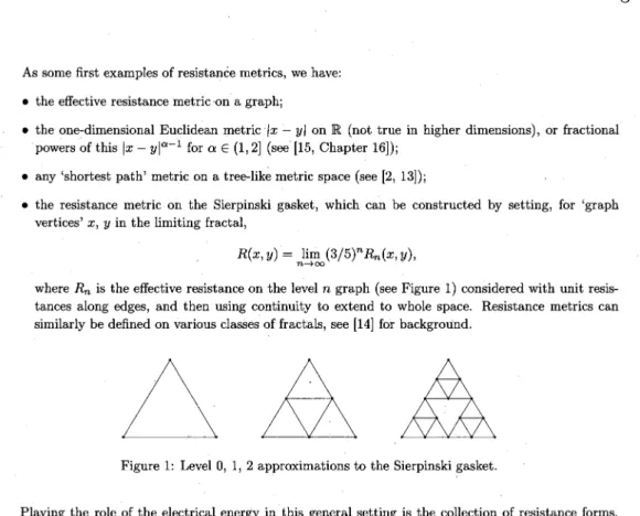
13

\bullet the resistance metric on the

_{Sierpinski gasket,}

which can be constructed

_by

_setting, for

_‘graph

vertices’ x, yinthe

limiting fractal,

R(x, y)=\displaystyle \lim_{n\rightarrow\infty}(3/5)^{n}R_{m}(x, y)

,

where_{R_{m}} isthe effectiveresistanceonthe leveln

_graph

(see

_Figure

1)

considered withunit resis‐

tances

_{along edges,}

and then

using continuity

toextend towholespace. Resistance metrics can

similarly

be definedonvariousclasses of

fractals,

see

[14]

for

background.

Figure

1: Level0, 1,2approximationstothe

Sierpinski gasket.

Playing

the role of the electricalenergy inthis

general setting

isthe collection ofresistanceforms. Wenow statethe definition of such

_objects.

Whilst this is _quitetechnical andwewill not discuss the role of thevariousconditionsindetail

_{here, importantly}

it

_gives

aroute to connecttheresistance metric

with astochasticprocess.

Definition 3.2

_([14,

Definition

_2.3.1]).

Let F be a set. A_pair

_{(\mathcal{E}, \mathcal{F})}

is a resistance

form

on X

if

it

satisfies

the

_followzng

conditions:

RF1 \mathcal{F} is alinear

subspace of

the collection

offunctions

\{f:F\rightarrow \mathbb{R}\}

_{containing constants,} and\mathcal{E} isa

non‐negative symmetric

quadratic form

on\mathcal{F} such that

\mathcal{E}(f, f)=0

if

and

only if f

is constanton F.

RF2 Let\sim be the

_equivalence

relation on\mathcal{F}

defined by saying f\sim g if

and

only if f-g

is constanton F. Then

_{(\mathcal{F}/\sim, \mathcal{E})}

is aHilbert_space.

RF3

_If

_{x\neq y}

, then there exists an

f\in \mathcal{F}

such that

f(x)\neq f(y)

.

RF4 Forany x,

y\in F,

\displaystyle \sup\{\frac{|f(x)-f(y)|^{2}}{\mathcal{E}(f,f)}:f\in \mathcal{F}, \mathcal{E}(f, f)>0\}<\infty.

RF5

_If

_{\overline{f}:=(f\wedge 1)\vee 0}

, then

f\in \mathcal{F}

and

\mathcal{E}(\overline{f},\overline{f})\leq \mathcal{E}(f, f)

for

any

f\in \mathcal{F}.

The

_following

theoremconnectsthenotionsofaresistance metricandaresistance

_form,

and

_yields

the stochasticprocessthat will be ofinterest inthe remainder of the article. In

particular,

it

_explains

how the

correspondences

stated at the end of theprevioussectionextendto themore

general

_present

setting. For

_simplicity

of the statement,we restrictto thecompactcase. Itisalso

possible

to extend the resultto

locally

compactspaces,

though

thisrequiresa morecarefultreatmentof the domain of the Dirichlet form.

Theorem 3.3

_([14,

Theorems_2.3.4,

_{2.3.6], [15,}

_Corollary

6.4 andTheorem

_{9.4]). (a)}

Let F be aset.

There is a one toone $\omega$

_wespondence

between resistance metrics and resistance

_forms

on F. This is

characterised

by

the relation:

R(x, y)^{-1}=\displaystyle \inf\{\mathcal{E}(f, f):f(x)=1, f(y)=0\}

(3.1)

for x\neq y

, and

R(x, x)=0.

(b)

Suppose

(F, R)

iscompactresistance metricspace, and $\mu$ is a

_finite

Borelmeasureon F

offull

_support. Then the

corresponding

resistance

_form

_{(\mathcal{E}, \mathcal{F})}

is a

regular

Dirichlet

form

on

L^{2}(F, $\mu$)

, andso

naturally

associated withaHunt_process

((X_{t})_{t\geq 0}, (P_{x})_{x\in F})

.

Asafirst

_example

oftheconnectionbetweenaresistance metricandastochastic_proCess

(beyond

the

example

of random walkson

graphs already

discussed),

consider

F=[0

,1

],

R=

Euclidean,

and $\mu$bea

finite Borelmeasureoffullsupporton

[0

,1

]

. Define

\displaystyle \mathcal{E}(f, g)=\int_{0}^{1}f'(x)g'(x)dx, \forall f, g\in \mathcal{F},

where \mathcal{F}=

_{{f\in C([0,1])}

:

f

is

absolutely

continuous and

f'\in L^{2} (dx)}.

Then

(\mathcal{E}, \mathcal{F})

isthe resistance

form associated with

_{([0,1], R)}

.

Moreover,

(\mathcal{E}, \mathcal{F})

isa

regular

Dirichlet formon

L^{2}( $\mu$)

.

Integrating by

parts

yields

\displaystyle \mathcal{E}(f, g)=-\int_{0}^{1}(\triangle f)(x)g(x) $\mu$(dx) , \forall f\in \mathcal{D}(\triangle) , g\in \mathcal{F},

where

_Af

_{=\displaystyle \frac{d}{d $\mu$}}

‐df,

and

_{\mathcal{D}(\triangle)}

contains those

f

such that:

_f'

existsand

df'

is

_absolutely

continuous with

respectto $\mu$,

$\Delta$ f\in L^{2}( $\mu$)

,and

f'(0)=f'(1)=0

. From

this,

we seethat if

$\mu$(dx)=dx

, then the Markov

process

naturally

associated with $\Delta$ isreflected Brownian motion on

[0

,1

]

.

(For

more

general

$\mu$_, the

relevant process is

simply

a

_{time‐change}

ofBrownianmotion

according

toRevuz measure _$\mu$.

)

_Taking

R(x, y)=|x-y|^{ $\alpha$-1}

for

_{$\alpha$\in(1,2],}

we canalso obtain $\alpha$‐stable_processesinthis _way

_{(see [15,}

_Chapter

16

4

_Scaling

limit

result

In this_section,wewill_presenta

_simplified

versionof the result establishedin

_[5],

theaim ofwhichwas

toestablish

_scaling

limits of stochastic

_processeg

associatedwith resistanceforms. In the full

_result,

\mathrm{a}

non‐explosion

conditionwas

provided

to extend from thecaseofcompactspacesthatweconsider here.

Moreover,

the resultwas also

_adapted

torandomspaces, and

incorporated spatial

\mathrm{e}

,mbeddings.

In

[9]

\mathrm{a} similar resultwas

proved

undermorerestrictive\mathrm{v}\mathrm{o}}\mathrm{u}\mathrm{m}\mathrm{e}

_growth

_conditions,whichwere

applied

tofurther deducea_convergencestatement

_regarding

the localtimesof theprocesses inquestion.

Tointroduce the result

_precisely,

letusfix the framework. In

particular,

wewrite

\mathbb{F}_{c}

for the collection of

_quadruples

of the form

_{(F, R, $\mu$, $\rho$)}

, where: F isanon‐empty set; RisaresistancemetriconF such

that

_{(F, R)}

is_{compact; $\mu$ is}a

locally

finite Borel

_regular

measureof full_support on

(F, R)

_; and p isa markedpointin F. Werecall that

saying

asequenceof suchspaces converges inthe

(marked)

Gromov‐

Hausdorff‐Prohorov

_topology

tosomeelement of_{\mathrm{F}_{c}}if all thespacescanbe

isometrically

embeddedinto

a commonmetricspace

(M, d_{M})

insuch a_waythat: the embedded _{sets converge}with respect to the

Hausdorff

_distance,

the embeddedmeasures_converge

weakly,

and the embedded marked_{pointsconverge.}

The

_following

result establishes

that,

ifsuch convergence occurs, then we also obtain _convergence of

stochastic_processes.

Theorem4.1

_{(cf. [5,}

Theorem

_1.2]).

_Suppose

that thesequence

(F_{n}, R_{\triangleleft n}, $\mu$_{n}, $\rho$_{n})_{n\geq 1}

in\mathrm{F}_{c}

satisfies

(F_{n}, R_{m},$\mu$_{n}, $\rho$_{n})\rightarrow(F, R, $\mu,\ \rho$)

(4.1)

inthe

_(marked)

_{Gromov‐Hausdorff‐Prohorov topology for}

some

(F, R, $\mu$, $\rho$)\in \mathbb{F}_{c}

. Itis then

possible

to

isometrically

embed

_{(F_{n}, R_{m})_{ $\gamma \iota$\geq 1}}

and

_{(F, R)}

intoa common _{metric space}

(M, d_{M})

insuch awaythat

weakly

as

probability

measures on

D(\mathbb{R}_{+}, M) (that

_is, the space

of cadlag

processes on M

equipped

with the usual SkorohodJ_{1}

‐topology),

where

_{((X_{t}^{n})_{t\geq 0}, (P_{x}^{n})_{x\in F_{n}})}

isthe Markovprocess

corresponding

to

(F_{n}, R_{n}, $\mu$_{n}, $\rho$_{n})

and

_{((X_{t})_{t\geq 0}(P_{x})_{x\in F})}

is the Markovprocess

corresponding

to

(F, R, $\mu$, $\rho$)

.

Ofcourse,

given

the

_{correspondence}

betweenmeasuredresistance metricspaces and stochasticpro‐

cesses,as describedinSection3, one

might intuitively

_expectthat Gromov‐Hausdorff‐Prohorovconver‐

gencewill

give

us all the informationweneedto obtainprocess convergence. To turn thisexpectation intoa

proof

we usethe fact

that,

for a_processassociated with aresistancemetric,wehavean

explicit

formula foritsresolvent kernel.

_(This

_{starting point}wasinfluenced

by

theoneusedasthe basis of the

corresponding

argumentfortrees in

_[2].)

In

particular,

for

_{(F, R, $\mu$, $\rho$)\in \mathrm{F}_{\mathrm{c}}}

,let

G_{x}f(y)=E_{y}\displaystyle \int_{0}^{$\sigma$_{x}}f(X_{s})ds

be the resolvent ofX killed on

_hitting

x wherewe have written $\sigma$_{x} for the

hitting

time ofx.

(NB.

Processesassociated withresistanceforms hit_points;the above_expressioniswell‐defined and

_finite.)

We then have that

G_{x}f(y)=\displaystyle \int_{F}g_{x}(y, z)f(z) $\mu$(dz)

where the resolvent kernel is_given

_by

g_{x}(y, z)=\displaystyle \frac{R(xy)+R(xz)-R(yz)}{2}.

(See [15,

Theorem

_4.3].)

In viewof this_expression,themetricmeasure_{convergence at}

(4.1)

_readily

_gives

convergenceof resolvents.

Relatively

standard arguments

subsequently yield semigroup

convergence,

whichinturn

_gives

_convergenceof finite dimensional distributions.

Togetfromconvergenceof finite dimensional distributionstoconvergence in

D(\mathbb{R}_{+}, M)

, it remains

tocheck

tightness

of theprocesses. For

this,

we

again

appeal

toan

explicit

expressionforaresolventin

termsof resistance. In

particular,

wehave for_anyclosedsetA that

g_{A}(yz)=\displaystyle \frac{R(y,A)+R(z,A)-R_{A}(y,z)}{2},

whereg_{A} is theresolvent kernel for theprocessX killedon

hitting

thesetA and

_{R_{A}(y, z)}

istheresistance

fromy tozwhen theset Ais \mathrm{s}\mathrm{h}\mathrm{o}\mathrm{r}\mathrm{t}\mathrm{e}\mathrm{d},i.e. in

defining

the resistancebetween yandz

similarly

to

(3.1),

weconsider

_only

functions thatareconstantonA.

(Again,

see

[15,

Theorem

_4.3].)

From

this,

andusing

thatX admits local times

_{(L_{t}(x))_{x\in F,t\geq 0}}

_(see

_[9

Lemma

_2.4])

that

satisfy

E_{y}L_{ $\sigma$ A}(z)=g_{A}(y, z)

where

$\sigma$ Aisthe

hitting

timeof A one canestablishviaMarkov’s

inequality

a

general

exittime estimateof the

form:

\displaystyle \sup_{x\in F}P_{x}(\sup_{s\leq t}R(xX_{s})\geq $\epsilon$)\leq\frac{32N(F, $\epsilon$/4)}{ $\epsilon$}( $\delta$+\frac{t}{\inf_{x\in F} $\mu$(B_{R}(x $\delta$))})

where

_{B_{R}(x $\delta$) :=\{y\in F : R(x, y)< $\delta$\}}

, and

N(F, $\epsilon$)

is the minimalsize ofan $\epsilon$ coverof F

(see [5

Lemma

_4.3]).

Theexactform of this

_expression

is not

_especially

_important.

_Rather,

thecrucialfactoris

the

_{straightforward dependence}

on

simply

metric‐measurequantities. Asa_consequence,wefind thatif

(4.1)

holds,

then

\displaystyle \lim_{t\rightarrow 0}\lim\sup_{xn\rightarrow\infty}\sup_{\in F_{n}}P_{x}^{n}(\sup_{\mathrm{s}\leq t}R_{m}(x, X_{s}^{n})\geq $\epsilon$)=0.

Tightness

of thesequenceX^{n} is thenastandard

application

ofAldous’

_tightness

criterion

_[12

Theorem 16.10and

_16.11].

5

_Applications

To

_complete

this

_overview,

we _present several

examples

to which the resistance metric frameworkis

5.1 Trees

Considera_sequenceof

_graph

trees

_{(T_{n})_{n\geq 1}}

,whereT_{n}hasvertex set

V(T_{n})

,shortest

path graph

distance

R_{n}

(noting

that this isaresistance

metric),

counting

measureonthe vertices_{$\mu$_{n}}

(placing

mass one on

each

_vertex),

androot_{$\rho$_{n}}.

Suppose

that forsomenullsequences

(a_{n})_{n\geq 1}, (b_{n})_{n\geq 1}

(V(Tn), a_{n}R_{m}, b_{ $\tau \iota$}$\mu$_{n}, $\rho$_{n})\rightarrow(TR, $\mu \rho$)

for somelimit in

\mathrm{F}_{c}

.

(NB.

Under the assumptions

stated,

(TR)

is aso‐called real

tree‘,

which isa

naturalmetric space

analogue

ofa

graph

tree.)

It then holds that

(X_{ta_{ $\tau \iota$}b_{n}}^{T_{n}})_{t\geq 0}\rightarrow(X_{t}^{T})_{ $\iota$\geq 0},

whereX^{T_{ $\tau \iota$}} is the random walk associated with

_{(V(Tn), R_{m}$\mu$_{n}$\rho$_{n})}

.

(Here

andinthe

examples below,

for the statementwe_supposethe_{state spaces}are

_{suitably isometrically}

embeddedintoa commonmetric

space.)

In

particular,

distributionalversions of theresult hold for:

Critical Galton‐Watsontreeswith finitevarianceconditionedon_size,

a_{n}=n^{1/2}b_{n}=n

. Versions

of the result for infinitevarianceGalton‐Watsontreesalso

hold,

see

[7].

The

_{(non‐lattice)}

_branching

random

walk,

where the

_underlying

tree isacritical Galton‐Watson treewith

_exponential

tails for the

offspring distribution,

and thestepshavea

centred,

continuous distribution with fourth order

_polynomial

tail

_decay

_[6].

\mathrm{e} _{\mathrm{A}‐coalescent}measuretrees

_[

2 Section

_7.5].

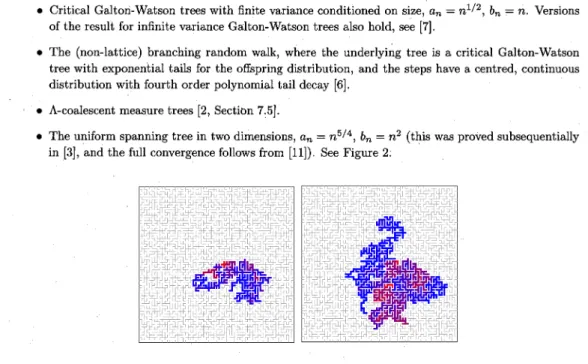
The uniform_spanningtreein two

_dimensions,

_{a_{n}=n^{5/4}b_{n}=n^{2} (this}

was

proved subsequentially

in

_[3],

andthefullconvergencefollows from

[11]).

See

Figure

2;

‐c

:.\vdash--\cdot ‐

Figure

2: Therangeofarealisation of the

simple

random walkonuniformspanningtreeon a 60\times 60

box

_(with

wired

_boundary

_conditions),

shown after _5,000and_{50,000 steps.} Frommost to least crossed

edges,

colours blend from redtoblue. Picture: Sunil‘ Chhita.

5.2

_Conjecture

for critical

_percolation

One model for whichan

appealing

_conjecturecanbe made istheincipientinfinite cluster of bond per‐

colation on

\mathbb{Z}^{d}

in

_{high dimensions,}

that _is, when d>6. In

particular,

it is

expected

thatthis model

satisfies thesame

_scaling

_propertiesas

branching

randomwalk,and thusone

might‘ anticipate

that ifIIC

isthe_incipient infinite cluster

_{(see [17]}

for a

construction),

R_{\mathrm{I}\mathrm{I}\mathrm{C}} isthe resistancemetric.onthis

(when

individual

edges

haveunit

_resistance)

and$\mu$_{\mathrm{I}\mathrm{I}\mathrm{C}} isthecountingmeasure onIIC,then the rescaled_sequence

satisfiesa

locally

_compact,distributionalversionof

_(4.1),

with limit

_being

_(an

unboundedversion

_of)

the

continuumrandomtree,andsothe associated random walks_convergetoBrownianmotiononthe latter

space, cf. theconjectureof

_[6].

See also therecent work of

_[4]

_regarding

the lattice

_branching

random

walk.

5.3

Critical random

_graph

One critical

percolation

model thatcan

already

be tackled with Theorem 4.1 isthat onthe

complete

graph.

In

_particular,

let

_G(n1/n)

be the

_{Erdós‐Rényi}

random

_graph

at

_criticality,

whichisobtained

_by

runningbond

percolation

with

edge

retention

_probability

_1/n

onthe

_{complete graph}

withnvertices. For

the

_largest

connectedcomponent

C_{1}^{n}

of

_G(n1/n)

itcanbe checkedthat

(C_{1}^{n}, n^{-1/3}R_{m}, n^{-2/3}$\mu$_{n}p_{n})\rightarrow(FR $\mu \rho$)

where the

limiting

spacecanbe described

explicitly,

cf.

[1].

_Hence,

as

_{originally proved}

in

_[8],

(X_{tn}^{n})_{t\geq 0}\rightarrow(X_{t})_{t\geq 0}.

5.4

_{Heavy‐tailed}

random conductance

model

on

fractals

Finally,

consider the

_{Sierpinski gasket graphs}

shown in

_Figure

1.

_Suppose

thatwe_equipthe

edges

of

these

_graphs

with

_random,

i.i.\mathrm{d}.

edge

conductances that

satisfy

P(c(x,y)\geq u)=u^{- $\alpha$}

forsome

$\alpha$\in(0,1)

. Onecanthen check thatresistance

homogenises,

inthesense

that, almost‐surely,

(V_{n}(3/5)^{n}R_{n})\rightarrow(F, R)

,

inthe Gromov‐Hausdorff

_topology,

where: V_{n}isthevertex setof the nth level

_graph,

R_{m}isthe effective

resistanceassociated with the random

conductances,

F isthe

_{Sierpinski gasket,}

and

_(up

toadeterministic

constant)

R is the effectiveresistanceonthe

Sierpinski gasket

introduced

above,

see

[9].

Recall from Section 2 that theVSRW associated with

_{(V_{n}R_{m})}

which has transition rates

_{$\lambda$_{xy}=}

c(x, y)

istheprocess

corresponding

to

_{(V_{n}R_{m}$\mu$_{n})}

where

_{$\mu$_{n}(\{x\})=1}

. Since

3^{-n}$\mu$_{n}\rightarrow $\mu$

, where $\mu$ is

(\ln 3/\ln 2)

‐dimensional Hausdorffmeasure on

Sierpinski gasket,

itfollows thatp the VSRW X^{n} _converges

tothe standard Brownian motiononthe

gasket,

X say:

(X_{t5^{\mathfrak{n}}}^{n})_{t\geq 0}\rightarrow(X_{t})_{t\geq 0}.

On the other

hand,

the associated CSRW has transition rates

_{$\lambda$_{xy}=c(xy)/c(x)}

where

_c(x):=

\displaystyle \sum_{y:y\sim x}c(x, y)

. This

corresponds

to the space

(V_{n}R_{m}, \mathrm{v}_{n})

where

$\nu$_{n}(\{x\})=c(x)

:

Similarly

to the convergenceofi.i.\mathrm{d}.sumsto $\alpha$‐stable

subordinators,

itfurther holds that

$\nu$_{n}:=3^{-n/ $\alpha$}\displaystyle \sum_{x\in V_{f}}c(x)$\delta$_{x}\rightarrow $\nu$=\sum_{i}v_{i}$\delta$_{x_{i}},

in

_{distribution,}

where

_{\{(v_{i}, x_{i})\}}

isaPoisson_{point process}on

(0, \infty)\times F

with

_intensity

cv^{-1- $\alpha$}dv $\mu$(dx)

(for

some deterministic constant c

).

Hence the \mathrm{C}\mathrm{S}\mathrm{R}\mathrm{W}Y^{n}_say,

(and

indeedits_{jump chain,} which is

simply

the discretetime

_simple

random walkamongstthesame

conductances)

_converges:

(Y_{t(5/3)^{n}3^{n/ $\alpha$}}^{n})_{t\geq 0}\rightarrow(Y_{t})_{t\geq 0},

where the

limiting

process\mathrm{Y}isthe so‐called

Fontes‐Isopi‐Newman

(FIN)

diffusiononthe

limiting fractal,

which is the

_{time‐change}

of the Brownian motionX

_according

to Revuz measure \mathrm{v}. Theprocess Y

spends

positivetimeat atomsof $\nu$ which demonstrates the_persistenceof the

_trapping

on

_edges

of

high

conductance of the CSRWinthe limit

_(a

phenomenon

which the result of the_previous

_paragraph

shows

References

[1]

L.

_{Addario‐Berry,}

N.

Broutin,

and C.

Goldschmidt,

The continuumlimit

of

critical random

_graphs,

Probab.

Theory

Related Fields 152

₍₂₀₁₂₎

no. 3-4367-406.

[2]

S.

_Athreya,

W. \mathrm{L}"\""{o}" \mathrm{h}\mathrm{r} andA.

_Winter,

Invariance

_{principle for}

variable

speed

random walks on _trees, Ann.

_Probab.,

to_appear.

[3]

M.T.

_Barlow,

D.A.

Croydon,

andT.

_{Kumagai, Subsequential scaling}

limits

of simple

random walk onthe two‐dimensional

uniform

_{spanning tree,}45

₍₂₀₁₇₎

no. _1,4‐55.

[4]

G. Ben

_Arous,

M.

Cabezas,

andA.

_Fribergh,

_Scaling

limit

_for

theant ina

_{simple labyrinth, preprint}

availableatarXiv: 1609.03977.

[5]

D.A.

_{Croydon, Scaling}

limits

of

stochasticprocessesassociatedwithresistance

forms

preprintavail‐ ableat arXiv: 1609.05666.

[6]

—,

Hausdorff

measure

of

arcs and Brownian motion onBrownian

spatial

trees,Ann. Probab.

37

₍₂₀₀₉₎

no. 3 946−978.

[7]

— S

caling

limits.

for simple

random walksonrandom ordered

graph

trees,Adv.in

Appl.

Probab.

42

₍₂₀₁₀₎

no.2 528−558.

[8]

—

Scaling

limit

for

the randomwalkonthe

largest

connectedcomponent

of

thecritical random

graph,

PubLRes. Inst. Math. Sci.48

₍₂₀₁₂₎

no. 2 279−338.

[9]

D. A.

_Croydon,

B. M.

_Hambly,

and T.

_{Kumagai, Time‐changes of}

stochasticprocesses associated

withresistance

_forms,

_preprint availableatarXiv:1609.02120.

[10]

M.

_Fukushima,

Y.

Oshima,

andM.

_Takeda,

Dinichlet

forms

and _symmetricMarkovprocesses, ex‐ tended

ed.,

de

_Gruyter

Studiesin

_Mathematics,

vol. _19, Walter de

_Gruyter

&

_Co.,

_Berlin,2011.

[11]

N..Holden and X.

_Sun,

SLE as a

_mating

of

trees in Eudidean geometry, preprint available at

arXiv: 1610.05272.

[12]

O.

_Kallenberg,

Foundations

_of

modern

_probability,

second

_{ed., Probability}

andits

_Applications

_(New

York),

Springer Verlag,

New

_York,

2002.

[13]

J.

_Kigami,

Harmonic calculusonlimits

of

networks andits

application

to

dendrites,

J. Funct. Anal.

128

₍₁₉₉₅₎

no. 1 48−86.

[14]

—

Analysis

on

fractals, Cambridge

Thacts in

Mathematics,

vol.

143, Cambridge University

Press, Cambridge,

2001.

[15]

—, Resistance

forms,

quasisymmetricmaps andheat kernelestimates,Mem.Amer. Math. Soc.

216

_(2012),

no. 1015\mathrm{v}\mathrm{i}+132.

[16]

P.

_Tetali,

Random walks and the

_effective

resistance

of networks,

J. Theoret. Probab.4

₍₁₉₉₁₎

no. 1, 101−109.

[17]

R.vander Hofstad and A. A.

_Járai,

The incipient

infinite

cluster

for high‐limensional

unoriented

percolation,

J. Statist.

Pbys.

114

₍₂₀₀₄₎

no.3-4625-663.