Impacts of wind-evaporation feedback in outer
regions on tropical cyclone development
著者
Aono Kenji
学位授与機関
Tohoku University
Doctoral Thesis
博士論文
Impacts of wind-evaporation feedback in outer regions
on tropical cyclone development
台風の外側における風蒸発フィードバックが
発達に及ぼす影響
青野 憲史
Doctoral Thesis
博士論文
Impacts of wind-evaporation feedback in outer regions
on tropical cyclone development
台風の外側における風蒸発フィードバックが
発達に及ぼす影響
東北大学大学院理学研究科
地球物理学専攻
Kenji Aono
青野 憲史
論文審査委員
山崎 剛 教授(指導教員・主査)
早坂 忠裕 教授
森本 真司 教授
伊藤 純至 准教授
岩崎 俊樹 教授(特)
2020
令和
2 年
Impacts of wind-evaporation feedback in outer regions
on tropical cyclone development
Abstract
It is important to understand the intensification processes of tropical cyclones (TCs) for pursuing predictability of TCs and assessment of their impacts. Unfortunately, the large amount of uncertainty remains in the recent operational forecasting systems, especially due to the rapid intensification (RI). The RI is considered to be a self-amplifying intensification process (i.e., positive feedback). It is well known that the dominant factor in the development of TCs is diabatic heating by water vapor condensation in the eyewall, and the water vapor source is evaporation from the sea surface. Since the amount of sea surface evaporation is assumed to be dependent on the surface wind speed, it is crucial to clarify the process of the feedback between the surface wind speed and evaporation from the sea (i.e., wind-evaporation feedback).
In Chapter 2, we revisit some persuasive theories of the TC intensification to address their drawbacks, and the concept of the conventional feedback processes: the conditional instability of the second kind (CISK), cooperative intensification theory, and the wind-induced surface heat exchange (WISHE). It has been widely considered that TCs are able to develop quickly with the positive feedback between the TC wind and local evaporation such as WISHE. However, in recent years, observational and numerical studies have pointed out that the contribution of local evaporation may be overestimated. These results also show that the primary water vapor source is inward water vapor flux from the outside of TCs. For this reason, there is no unified theory to resolve the conflicts between them. The second section describes the bulk method of the sea surface water vapor flux which is assumed to be a function of the surface wind speed and water vapor difference at the air-sea interface. We show the concerns for the wind-evaporation feedback focused on local evaporation. The third section the surface friction which induces convergence near the surface.
In Chapter 3, we examine the roles of water vapor flux across the air-sea interface in the outside TC (i.e., light wind region) on the TC development. Using the three-dimensional cloud-resolving nonhydrostatic atmospheric model (JMA-NHM), we perform four idealized
Thesis Adviser
Dr. Takeshi Yamazaki
Author
ii
experiments in which a TC-like vortex is given to a horizontally uniform environment field. In order to remove the wind speed dependence on the surface water vapor flux outside of the TC, we introduce the lower limits of the 10-m wind speed in calculation of water vapor flux (5, 10, and 15 m s−1). Results show that increasing the lower limit reduces the radial water vapor contrast
in the lower troposphere (below 100 m) and suppresses the TC size and intensity at the mature stage by 30%–33% and 5%–14%, respectively, compared to the control run. The increased evaporation enhances the outer convective activity and reduces the radial pressure gradient in the lower troposphere. Consequently, the secondary circulation becomes weak and narrow because the inflow flux is blocked by the convections outside the TC. Moreover, the outer region convection suppresses the rainband activity, within a radius of 300 km from the TC center. It is assumed that the wind-evaporation feedback plays a crucial role in sustaining the secondary circulation and promotes the spin-up.
In Chapter 4, we investigate the wind-evaporation feedback in the outside TC from a case study for TC Hagibis in 2019 because the hypothesis suggested in Chapter 3 have some concerns that the idealized environment ignores various factors such as a vertical shear, steering flow, and non-uniform thermodynamic field. In addition, there is no proof that whether the initial vortex is consistent with the realistic structure of a TC. We pick up TC Hagibis (2019) because of its high intensification rate (100 kt day−1, according to the Joint Typhoon Warning Center). Similar to the
experimental design in Chapter 3, we apply a lower limit into the bulk formula to cut off the wind-evaporation feedback outside Hagibis (2019). We perform two sensitivity experiments using the same model in Chapter 3, JMA-NHM: the control run with no limits (CTL), and disabled feedback run with a lower limit of 10 m s−1 (MIN10). The derived results show some inconsistencies with
the findings in Chapter 3. The intensity in the CTL run was smaller than that in the MIN10 run, and its RI onset was 6 hours behind the MIN10’s onset. Besides, the intensification rate in MIN10 is larger than that in CTL. The analysis of water vapor budget in the inner core of the simulated TC reveals that the dominant source of water vapor for the TC development is the horizontal inward moisture flux. The contribution of the sea surface moisture flux is less than 5% of the horizontal inward flux after the onset of intensification. In MIN10, the water vapor convergence becomes large earlier, resulting in the stronger intensity of the simulated TC. Considering that there is the wide and robust inflow layer to TC Hagibis (2019) at the initial condition, it is simulated that the TC early gathers the large amount of water vapor from the excessive evaporation at the sea surface with the weak wind. Thus, it is the reasons why the MIN10 experiment performed the stronger TC without the wind evaporation.
In summary, the present thesis points out that the radial contrast of water vapor near the surface is important for the TC organization than the amount of water vapor itself. The radial contrast of water vapor field is more crucial than the CISK paradigm. In addition, the dominant
iii
role of the horizontal moisture flux suggests that it is insufficient to diagnose the maximum potential intensity (MPI) of TCs based on the WISHE paradigm which consists of only eyewall (and outflow layer) information. Based on the idealized experiments, we propose the new hypothesis of the wind-evaporation feedback. Our findings give a very different interpretation of the wind-evaporation feedback on the TC development from the conventional ideas.
Lastly, we have to mention some issues for further progress. First of all, the concern is the inconsistency of the results from the idealized simulation (Chapter 3) and real case simulation (Chapter 4). In the real case experiments, the sea surface evaporation outside the TC results in earlier intensification. Since the reason is considered to be the initial conditions or the case dependency, it is insufficient to prove our hypothesis from the single case study. To verify the general roles of suppressing sea surface evaporation outside TCs, it is necessary to use the statistical approach. Next, in relation to the above, it is to construct the explanatory variable based on the radial contrast of water vapor into the statistical intensity prediction models. These models use atmospheric and/or oceanic parameters to predict the intensity change of TCs. Based on the new wind-evaporation feedback hypothesis, the radial distribution of water vapor (or sea surface latent heat flux) is listed as the candidates of the explanatory variable. Considering that convections outside the TC block the water vapor transport to the TC system, it is favorable for the TC intensification that the atmospheric conditions in the outer regions are convective stable. Thus, the indication of the stability of the atmosphere, such as convective inhibition (CIN) and the distribution of outgoing long-wave radiation (OLR), is also considered to be explanatory variable. We would like to assess the predictability and the contribution of new explanatory variables to the total intensity change. If these issues are cleared, it will bring more improvement in the forecast accuracy.
iv
Contents
Abstract
i
List of Figures
vi
List of Tables
ix
Acknowledgements
x
1 Introduction
1
1.1
Background of Tropical Cyclone Prediction... 1
1.2
Purpose of This Study ... 4
2 Wind-Evaporation Feedback on TC Intensification
5
2.1
Revisiting the Main Paradigms ... 5
2.1.1
CISK ...5
2.1.2
Cooperative Intensification ...7
2.1.3
WISHE ...7
2.2
Sea Surface Evaporation ... 8
2.3
Modeling of Sea Surface Friction ... 9
2.3.1
Drag Coefficient ...9
2.3.2
Sea Surface Roughness ... 10
3 Impacts of Wind-Evaporation in Outer Regions from Idealized Simulations
(Aono, K., T. Iwasaki, and T. Sasai, 2020: Effects of wind-evaporation feedback
in outer regions on tropical cyclone development. J. Meteor. Soc. Japan, 98, 319–
v
3.1
Introduction ... 11
3.2
Method ... 12
3.3
Results... 14
3.4
Discussion ... 20
3.4.1
TC Intensity ... 21
3.4.2
TC Size ... 23
3.5
Conclusions ... 23
4 Case Study: TC Hagibis (2019)
26
4.1
Introduction ... 26
4.2
Experimental Design ... 28
4.2.1
Model Setup ... 28
4.2.2
Input Data ... 28
4.2.3
Sensitivity Experiments ... 28
4.3
Results and Discussion ... 31
4.3.1
Validation of Control Simulation ... 31
4.3.2
Evaluation of the Sensitivity Experiments ... 32
4.4
Summary and Conclusions ... 38
5 Concluding Remarks
40
vi
List of Figures
1.1 Tracks of TCs during 2011–2015 using the best track dataset archived at the Japan Meteorological Agency (JMA). Black line depicts the path of each TC. Color dots on the line denote the position of the TC center every 6 hours. The dot color corresponds to the intensity. Note that the tropical depression and extratropical cyclone are not classified into the TC. ...2 1.2 Annual-average errors of JMA’s operational forecasts of TC intensity in terms of the
minimum sea-level pressure (top) and the maximum wind speed (bottom). From Yamaguchi et al. (2018). ...3 2.1 A schematic image in the TC-centered cylindrical coordinates. Green arrow
represents the primary circulation, and blue arrows depict the secondary circulation. Orange shading shows the amount of wind-induced evaporation from the sea which is largest at the radius of maximum wind (RMW) on the surface. ...6 3.1 Values of the surface water vapor exchange coefficient under the value of Vq. Four
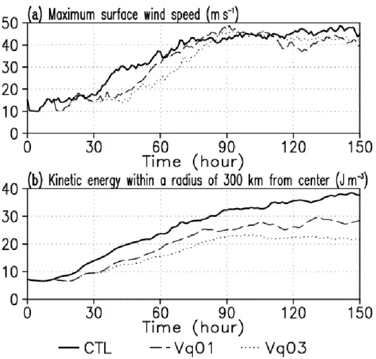
lines show CTL (solid), Vq05 (broken), Vq10 (dotted), and Vq15 (chain). ... 14 3.2 Temporal variations in maximum surface wind speed (a), area-averaged kinetic
energy within a radius of 300 km from the TC center (b), and 17 m s−1 wind radius at
420 m height (c). Results are derived from CTL (solid line), Vq05 (broken line), Vq10 (dotted line), and Vq15 (chain line). The horizontal axis shows the TC development from the initial state. ... 15 3.3 Radius–time cross sections of azimuthally averaged precipitation (shade, mm h−1)
and surface wind speed (contour, 5 m s−1 interval) for CTL (a), Vq05 (b), Vq10 (c),
and Vq15 (d). The horizontal axis shows the distance from the TC center. The vertical axis shows the time variation from the initial state... 16 3.4 Vertical structures of radial (a–d), vertical (e–h), and tangential wind speeds (i–l)
averaged in the mature (T = 90–150 hr) stage for CTL (a, e, i), Vq05 (b, f, j), Vq10 (c, g, k), and Vq15 (d, h, l). Horizontal and vertical axes show distances from the TC center and altitude, respectively. ... 17 3.5 Warm core structures averaged in the mature stage (T = 90–150 hr) for CTL (a), Vq05
vii
(b), Vq10 (c), and Vq15 (d). Horizontal and vertical axes show distances from the TC center and altitude, respectively. ... 18 3.6 Equivalent potential temperature (EPT) averaged in the lower troposphere (0–100 m)
in the developing (T = 30–90 hr) (a) and mature (T = 90–150 hr) (b) stages. Four lines show CTL (solid), Vq05 (broken), Vq10 (dotted), and Vq15 (chain), respectively. ... 19 3.7 Mass streamfunction (contour, 1.0 × 10⁸ kg s−1 interval) and relative humidity
(shade, %) for four experiments in the developing (a, c, e, g) and mature (b, d, f, h) stage for CTL (a, b), Vq05 (c, d), Vq10 (e, f), and Vq15 (g, h). Mass streamfunction represents secondary circulation. ... 20 3.8 Temporal variations in maximum surface wind speed (a) and area-averaged kinetic
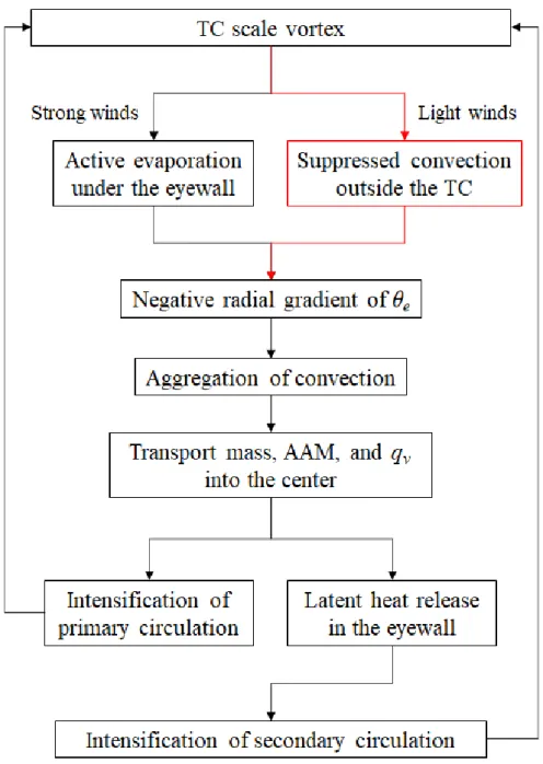
energy within a 300 km radius from the TC center (b). Results are derived from CTL (solid line), Vq01 (broken line), and Vq03 (dotted line). The horizontal axis shows the TC development from the initial state. ... 22 3.9 Schematic diagrams of the roles of the radial contrast of water vapor mixing ratio in
TCs. These diagrams show secondary circulations of TCs with (left) and without (right) the wind-evaporation process in the outer region. The orange shadings represent the water vapor mixing ratio significantly controlled by the surface evaporation. The blue shade arrows represent the strength of the secondary circulation. The circles with an inscribed X denote the TC’s tangential winds into the page and their size correspond to the wind speed). ... 24 3.10 Schematic diagram of the updated wind-evaporation feedback hypothesis. The
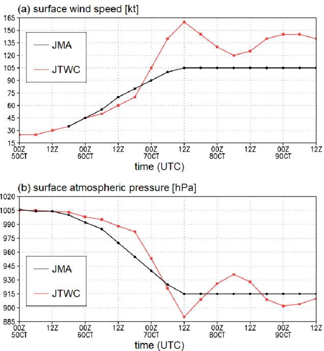
process in which the surface light winds suppress convection outside the TC plays the role of keeping the negative gradient of water vapor (red lines). ... 25 4.1 Intensity of TC Hagibis (2019) in terms of the maximum surface wind speed (a) and
the minimum surface pressure (b) archived at JMA (black), and JTWC (red). Note that wind speed is recorded in knots (1 kt ~ 0.5144 m s−1). ... 27
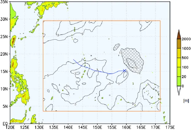
4.2 Track of Hagibis (2019) in the integration period (blue line; 1200 UTC 5 Oct–1200 UTC 8 Oct). The blue cross symbol indicates the Hagibis’s center observed by JMA at 1200 UTC on 5 October. The orange box represents the numerical domain. Black contour lines indicate the wind speed at the lowest model level (20-m height) at the initial time, and the hatched area denotes where its speed is larger than 10 m s−1.
Shading shows the elevation from GTOPO30... 29 4.3 Schematic diagram of the disabled feedback run with a lower limit of Vq. Shading
with orange color indicates the region where the 10-m wind satisfies V10 ≤ Vq. ... 31
4.4 Time series of intensity in terms of the maximum surface wind speed (a) and the minimum surface pressure (b) derived from CTL (black line) and MIN10 (red line)
viii
run. Blue cross symbols show the intensity archived at the JMA best track. Three vertical dotted lines indicate the onset of RI in CTL (black), and MIN10 (red), respectively. The time intervals of each data are 6-hourly for the best track, and 3-hourly for CTL and MIN10. ... 32 4.5 Tracks of simulated TCs and best track of Hagibis (2019). The black (red) line depicts
the path in the CTL (MIN10) run. The opened circles, squares, and blue cross symbols indicate the locations of Hagibis (2019) from CTL, MIN10, and best track, respectively, every 6 hours in the integration period (i.e., 1200 UTC 5 Oct–1200 UTC 8 Oct). The shading shows the 3-day averaged (5–7 October) SST calculated from daily HIMSST. The box with broken thick lines shows the numerical domain. ... 33 4.6 Comparisons of ERA5 (a, c) and CTL (b, d) for daily averaged latent heat flux (shade),
geopotential height at 850-hPa surface (contour, 60 m interval), and horizontal winds at 925-hPa surface (vectors) on 6 October (a, b) and 7 October (c, d). Wind speeds of less than 1 m s−1 are omitted. ... 34
4.7 Time series of size in terms of the radius of maximum wind (RMW; a), the radius of 15 m s−1 wind speed (R15; b), and the radius of 10 m s−1 wind speed (R10; c) derived
from CTL (black line) and MIN10 (red line) run. ... 35 4.8 Similar to Fig.4.6, but from the MIN10 run on 6 October (left) and 7 October (right).
... 36 4.9 Time series of domain-averaged total precipitable water (a), and accumulated rainfall
(b) derived from the CTL (black line), and MIN10 (red line) run. ... 37 4.10 Time series of the vertical integral of horizontal (a), and surface (b) water vapor flux
within an 80-km radius of the center derived from CTL (black line) and MIN10 (red line) run. The horizontal water vapor flux is vertically integrated from the surface to 1-km height. ... 38
ix
List of Tables
2.1 Constants for calculating the drag coefficient. Note that the constants above 50 m s−1
are extrapolated from the values in the range from 25 m s−1 to 50 m s−1 because it is
undefined in the original model (Kondo 1975). ...9 4.1 Model settings. GSM: global spectral model, HIMSST: high resolution merged
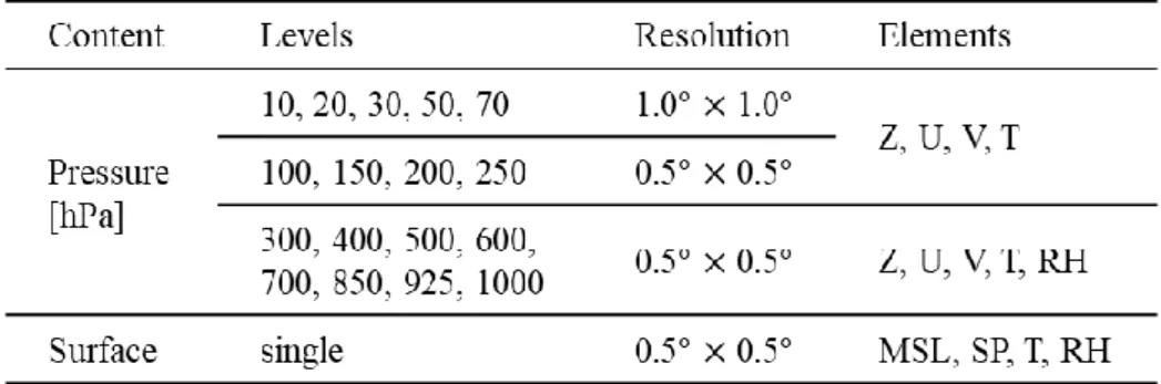
satellite and in-situ data sea surface temperature, GTOPO30: a global digital elevation model with a horizontal grid spacing of 30 arc seconds. ... 30 4.2 List of GSM variables. Z: geopotential height, U: eastward wind speed, V: northward
wind speed, T: temperature, RH: relative humidity, MSL: mean sea level pressure, SP: surface pressure. ... 30
x
Acknowledgements
First of all, I would like to express my sincere appreciation to Prof. Takeshi Yamazaki and Res. Prof. Toshiki Iwasaki for their guidance and supports throughout my doctoral course. Their lectures and advices always encourage me.
I show my gratitude to Dr. Takahiro Sasai for his support of me about not only the research but also private. His recommendation always guided me through many difficulties. I could not publish this doctoral thesis without his supports.
I express my deep respect to Dr. Ryuhei Yoshida and Dr. Shota Ishii. They taught me attitudes for the future and as a scholar early in my master course.
I show special thanks to Assoc. Prof. Shusaku Sugimoto whose constructive comments with expertise in Oceanography and Meteorology on my study. His outstanding vision brought me many ideas for my study.
Here, I express my deep appreciation to persons who were of great help in supporting my work, individually. Dr. Shin Fukui helped me ever since the first year of the Tohoku University. Dr. Irina Melnikova gave profitable days through discussion on the various topic as well as Meteorology. Ms. Saeko Hasebe helped my office work for many times.
I thank the Japan Meteorological Agency (JMA) for permission to use the Non-Hydrostatic Model (NHM), and the Cyberscience Center, Tohoku University for providing supercomputing resources.
Lastly, I will dedicate this thesis to my family. They agreed my entering the graduate school and have supported me for a long time.
1
Chapter 1
Introduction
1.1 Background of Tropical Cyclone Prediction
The understandings of the three-dimensional structure and developing mechanism of tropical cyclone (TC) is still one of the important issues for tropical and subtropical Meteorology. TCs are mesoscale (on the order of about 1000–2000 km in diameter) phenomena with the aggregation of small scale deep convective clouds, and can sometimes last over five days. The coastal countries and regions have often experienced devastating damage from strong winds, heavy rainfall, and storm surge due to TCs (e.g., Beven et al. 2008; Coronel et al. 2016; Hatsuzuka et al. 2020; Kawabata et al. 2012; Takemi and Unuma 2020) (Fig. 1.1). In addition to these hazards, TCs have potential to affect the global climate through multi-scale interactions (e.g., an interaction between a TC and midlatitude flow; Archambault et al. 2013, 2015; Bosart et al. 2012), vertical transport of water vapor or chemical species to the upper troposphere/lower stratosphere (Allison et al. 2018; Preston et al. 2019; Ray and Rosenlof 2007), and a sea water heat pump (Sriver and Huber 2007, 2010).
The accuracy of the track forecasts is fundamental to the TC prediction. The primary force to drive the TC is the environmental flow (steering flow; Chan and Gray 1982) (in the western North Pacific, the westerlies, subtropical high, and trade winds). Due to improvements in numerical weather predictions and developments of forecasting techniques, annual-average track errors have significantly decreased (Heming et al. 2019; Kawabata and Yamaguchi 2020; Magnusson et al. 2019; Titley et al. 2020; Yamaguchi et al. 2017). However, many studies reported the interaction between a TC and its environment (e.g., Ito et al. 2020; Iwasaki et al. 1987; Sun et al. 2015). In order to reveal the interaction, it is necessary to understand the TC structure during its life cycle. Compared with the operational track forecast errors, the forecast errors of intensity have not been improved (Fig. 1.2). Besides, forecasts have generally underestimated the TC intensities
1.1. BACKGROUND OF TROPICAL CYCLONE PREDICTION 2
(Yamaguchi el al. 2017). Why did the prediction of TC intensity show little improvement? Ito (2016) reported that intensity errors tend to be larger in the rapid intensification (RI) phase of TCs in the western North Pacific and the South China Sea. Recently, Trabing and Bell (2020) found that the rapid weakening events also have caused larger errors in the Atlantic and the east Pacific. According to Liang et al. (2016), note that the rapid weakening events can occur in favorable environments over the sea. These facts show that the recent operational forecasting systems cannot yet predict the rapid intensity change.
In terms of the predictability of RI events, the self-amplifying intensification system (positive feedback) should be fully understood. Many studies discussed the air-sea interaction as a part of feedback. It is generally accepted that the source of water vapor which intensifies the TC circulation is the underlying warm sea. Besides, most of the numerical models hypothesize that Figure 1.1: Tracks of TCs during 2011–2015 using the best track dataset archived at the Japan Meteorological Agency (JMA). Black line depicts the path of each TC. Color dots on the line denote the position of the TC center every 6 hours. The dot color corresponds to the intensity. Note that the tropical depression and extratropical cyclone are not classified into the TC.
1.1. BACKGROUND OF TROPICAL CYCLONE PREDICTION 3
surface winds control water vapor transfer across the air-sea interface. In other words, the stronger surface winds promote evaporation from the sea. Therefore, it is possible to activate the positive feedback which called as the wind-evaporation feedback. However, that feedback inside the TC alone causes inconsistency with observation facts and the water budget analysis. Although these Figure 1.2: Annual-average errors of JMA’s operational forecasts of TC intensity in terms of the minimum sea-level pressure (top) and the maximum wind speed (bottom). From Yamaguchi et
1.1. BACKGROUND OF TROPICAL CYCLONE PREDICTION 4
details are described later, briefly speaking, it is insufficient to explain a long-lasting TC structure and precipitation by only the wind-evaporation feedback under the eyewall. There is no unified theory yet to resolve the conflicts between them.
1.2 Purpose of This Study
In this thesis, we investigate the wind-evaporation feedback especially outside TC using the three-dimensional cloud-resolving nonhydrostatic atmospheric model, JMA-NHM, and propose new insights into the feedback for the TC developing. Our interests in this study are as follows:
⚫ How does the wind-controlled evaporation outside the TC affect the intensification? ⚫ If the water vapor transport into the TC is crucial, what is the favorable water vapor
distribution for the development?
⚫ How does the TC intensify with the wind-evaporation feedback?
Chapter 2 revisits the main spin-up paradigms to introduce the concept of the wind-evaporation feedback. Chapter 3 shows the impacts of convections induced by wind speed independence outside the idealized TC, and assumes the wind-evaporation feedback outside the TC to be playing roles to develop the secondary circulation, which results in increasing the intensity. To confirm that hypothesis, Chapter 4 presents the response under the real atmospheric conditions, a case of TC Hagibis in 2019, and constructs the wind-evaporation feedback process. Chapter 5 summarizes the findings and outlooks for future works.
5
Chapter 2
Wind-Evaporation Feedback on TC
Intensification
2.1 Revisiting the Main Paradigms
In the TC-centered cylindrical coordinates, a TC has two fundamental circulations called as the primary circulation and secondary circulation, respectively (Fig. 2.1). The primary circulation corresponds to the tangential winds, which induce a large amount of water vapor from the sea under the eyewall. From the axisymmetric view, the secondary circulation consists of flows in the radius-height cross section. The radial inward flow in the lower troposphere transports water vapor and absolute angular momentum (AAM) into the TC center. The previous spin-up theories are based on either or both of these two circulations.
In this section, we revisit some representative theories to introduce the wind-evaporation feedback process for the TC intensification with special attention to the outside of TCs. Here, we review following typical spin-up paradigms:
⚫ the conditional instability of the second kind (CISK);
⚫ the cooperative intensification; and
⚫ the wind-induced surface heat exchange (WISHE).
2.1.1 CISK
The conditional instability of the second kind (CISK) paradigm is an axisymmetric balance theory proposed by Charney and Eliassen (1964). This paradigm is a kind of the cooperative interaction mechanism and focuses on surface friction, which acts to supply moisture to the TC. CISK
2.1. REVISITING THE MAIN PARADIGMS 6
assumes that diabatic heating by deep cumulus convection in the eyewall is proportional to moisture convergence. Therefore, the self-amplifying intensification system in the CISK mechanism is considered to be the positive feedback between frictional convergence and convection. Note that CISK does not necessarily include the air-sea interaction (Craig and Gray 1996; Ooyama 1969, 1982).
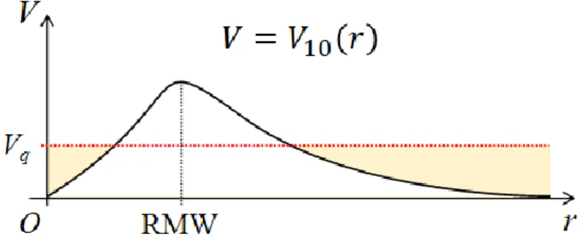
Craig and Gray (1996) refuted the CISK paradigm because the TC development was sensitive to the bulk coefficients for sensible and latent heat flux using an axisymmetric nonhydrostatic model. Their results also showed that the response of the drag coefficient to the intensification rate was not clear. Therefore, according to Craig and Gray (1996), frictional convergence works as an energy sink. Furthermore, since CISK was constructed without moistening process from the underlying sea, the intensification rate depends on initial surrounding convective available potential energy (CAPE). However, it is insufficient in the CISK mechanism to capture the observed intensification rate because the initial CAPE is too small to sustain the secondary Figure 2.1: A schematic image in the TC-centered cylindrical coordinates. Green arrow represents the primary circulation, and blue arrows depict the secondary circulation. Orange shading shows the amount of wind-induced evaporation from the sea which is largest at the radius of maximum wind (RMW) on the surface.
2.1. REVISITING THE MAIN PARADIGMS 7
circulation. Indeed, Ooyama (1982) already mentioned that the CISK assumption is unrealistic especially in the early developing stage.
2.1.2 Cooperative Intensification
The cooperative intensification paradigm (Ooyama 1969) is similar to CISK (Charney and Eliassen 1964) but the crucial difference between them is water supply. Ooyama (1969) assumed that diabatic heating released by convections generated the vertical mass flux which connected the inflow layer and outflow layer. The intensification of convection near the TC center intensifies convergence (divergence) in the inflow (outflow) layer, and thus the TC can aggregate spontaneously more water vapor and AAM. In the cooperative intensification theory, it is essential to estimate the temporal evolution of convective instability for derivation of the steady-state TC. Besides, Ooyama (1969) recognized the importance of the surface moisture flux in maintaining convective instability.
2.1.3 WISHE
The fundamental concept of the wind-induced surface heat exchange (WISHE) paradigm is based on the air-sea interaction instability (Emanuel 1986, 1989). Emanuel (1986) derived the thermal wind balance assuming that equivalent potential temperature (EPT) and AAM were conserved in the eyewall. In the WISHE paradigm, considering that EPT and AAM in the free atmosphere are controlled by the sea surface fluxes, the feedback steps work as follows. At first, if the sea surface entropy flux increases, then the radial gradient of EPT in the eyewall updraft becomes sharp. Second, to satisfy the thermal wind balance the tangential wind at the top of the boundary layer becomes stronger, and then the surface wind increases due to the turbulence in the boundary layer. Finally, the intensified surface wind promotes evaporation from the sea surface.
From the idea of the air-sea interaction instability, it is possible to derive a reachable intensity under the thermodynamic environment at the certain time. That upper bound is called as maximum potential intensity (MPI). Recently, Rousseau-Rizzi and Emanuel (2019) developed the WISHE theory and introduced the new surface MPI with a few assumptions. Summarizing the multiple versions (Rousseau-Rizzi and Emanuel 2019), the WISHE-based MPI is determined by the local surface flux at the eyewall and the temperature of the outflow layerfar outside the center.
2.2. SEA SURFACE EVAPORATION 8
2.2 Sea Surface Evaporation
In the numerical models, the water vapor transfer at the sea surface, Fq, is parameterized using
bulk formula as follows,
𝐹𝑞 = −𝐶𝑞𝑉10(𝑞𝑣− 𝑞𝑣𝑠), (2.1)
where Cq is the bulk transfer coefficient, V10 is wind speed at a height of 10 m, qv is specific
humidity, and qvs is saturated specific humidity at the sea surface temperature (SST). Assuming
the constant Cq (e.g., Bell et al. 2012), Eq. (2.1) becomes a function of the surface wind speed
and water vapor difference at the air-sea interface. Therefore, if the values of water vapor disequilibrium (∆q = qv − qvs) are same, then the amount of evaporation from the sea surface is
proportional to the surface wind speed (i.e., wind-evaporation). The wind-evaporation forms the local evaporation at the radius of maximum wind (RMW) (Fig. 2.1). Therefore, we obtain that the self-amplifying intensification in WISHE is the positive feedback between the local evaporation and primary circulation.
However, observational and numerical studies have claimed the impact of local evaporation to be overestimated. Makarieva et al. (2017) analyzed satellites, reanalysis, and best track datasets and found that local evaporation alone was impossible to sustain a TC’s rainfall. Using the idealized simulation with an axisymmetric model, Kurihara (1975) calculated that evaporation at the surface accounted for ~26% of the flux convergence within a 500-km radius for the energy budget. Yang et al. (2011) estimated evaporation from the sea at 11% (5.5%) of the inward horizontal vapor transport within a 150-km radius (in the inner core, within a 50-km radius) from the TC center for the case of TC Nari (2001) using a numerical simulation at high resolution (2-km grid spacing). Fritz and Wang (2014) conducted different model with a four-grid nested domain (1 km in the innermost domain) for Tropical Storm Fay (2008) and showed that the contribution of local evaporation dropped to 12% after the Fay’s genesis. They concluded (p. 4331) that the inward water vapor flux was the primary source while the local evaporation made a small contribution but “... plays an important, but not dominant, role in replenishing the column moisture when convection is inactive and the low-level convergence is relatively weak.” From these facts, they suggested the positive feedback between the primary circulation and secondary circulation.
2.3. MODELING OF SEA SURFACE FRICTION 9
2.3 Modeling of Sea Surface Friction
As described above, the sea surface friction performs dual parts of the TC development, energy source or sink. In this section, we describe only the drag coefficient over the sea because the bulk coefficients for the water vapor and sensible heat fluxes are assumed to be constant with the surface wind speed throughout this thesis.
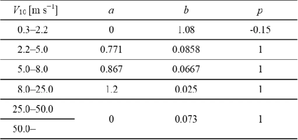
2.3.1 Drag Coefficient
According to the Kondo (1975) model, the drag coefficient Cm over the sea is parameterized using
the wind speed at a height of 10 m V10 as follows,
𝐶𝑚 = 10−3𝐴[𝑎 + 𝑏𝑉10
𝑝], (2.2)
where a, b, and p are constants summarized in Tab. 2.1, and A is a function of the stability S:
𝐴 = {
1 + 0.47√𝑆, 𝑆 ≥ 0
0.1 + 0.03𝑆 + 0.9 exp (4.8𝑆), −3.3 < 𝑆 < 0 0, 𝑆 ≤ −3.3
, (2.3)
Table 2.1: Constants for calculating the drag coefficient. Note that the constants above 50 m s−1
are extrapolated from the values in the range from 25 m s−1 to 50 m s−1 because it is undefined in
2.3. MODELING OF SEA SURFACE FRICTION 10 𝑆 = 𝑆0 |𝑆0| |𝑆0|+0.01, (2.4) 𝑆0= (𝜃𝑠− 𝜃)𝑉10−2[1 + log10( 10 𝑧)] −2 , (2.5)
where θ and θs are potential temperature at the lowest atmospheric level and the sea surface,
respectively, and z represents the height of the lowest atmospheric layer. From Tab. (2.1), in the TC where the surface wind speed is 15 m s−1, the drag coefficient increases with the surface wind
speed assuming an unstable condition (S ≥ 0) and relatively small change of (θs − θ).
2.3.2 Sea Surface Roughness
Using the above coefficients, Cm and A, sea surface roughness z0m is defined as
𝑧0𝑚 = 10 exp (−𝑘√ 𝐴
𝐶𝑚), (2.6)
where k is the von Karman constant (Kondo 1975). Under the above assumption, the surface friction increases with the drag coefficient Cm.
11
Chapter 3
Impacts of Wind-Evaporation in Outer
Regions from Idealized Simulations
3.1 Introduction
A main energy source for tropical cyclones (TCs) is latent heat release by condensation of water vapor from the underlying sea. There are some well-known TC intensification theories as described in Chapter 2. The first is the conditional instability of the second kind (CISK) theory (Charney and Eliassen 1964). Low-level frictional forcing induces inflow, which transports warm moist air in the direction of the TC center. The air mass convergence lifts the warm-moist air to the level of free convection and thereby initiates deep cumulus convection. Many authors have examined the sensitivity of the surface exchange coefficient for momentum (e.g., Montgomery et
al. 2010; Coronel et al. 2016). The second is the wind-induced surface heat exchange (WISHE)
mechanism proposed by Emanuel (1986); this is based on positive feedback between evaporation and the surface wind. The surface wind activates evaporation from the sea. The evaporated water from the sea induces convection near the eyewall, which intensifies the TC. Based on the WISHE mechanism, Emanuel (1986) reported the mature TC intensity and suggested the model of maximum potential intensity. In the developing stage, because the intensified wind evaporates more water from the sea, some studies have specifically examined the effect of introducing an upper limit to the surface entropy (sensible and latent heat) flux on the TC intensity: Montgomery
et al. (2009, 2015) reported that the effect of a capped flux is rather slight on the TC intensity.
They questioned WISHE. By contrast, results of recent studies have demonstrated that the capped
This chapter was published as Aono, K., T. Iwasaki, and T. Sasai, 2020: Effects of wind-evaporation feedback in outer regions on tropical cyclone development. J. Meteor. Soc. Japan, 98, 319–328, doi:10.2151/jmsj.2020-017.
3.2. METHOD 12
exchange coefficient reduces evaporation and suppresses deep convection near the eyewall, suggesting that the results support WISHE (Zhang and Emanuel 2016; Chavas 2017). As a result, an open question remains to be about the effects of the wind-evaporation feedback on the TC intensity.
Some studies have examined the role of surface flux or convection in the outer region on the TC intensity and structure (e.g., Bister 2001; Bister and Emanuel 1997; Kowaleski and Evans 2016; Lee and Chen 2014; Lin et al. 2015; Miyamoto and Takemi 2010; Rai et al. 2016; Sun et
al. 2013, 2014; Xu and Wang 2010). Bister and Emanuel (1997) and Bister (2001) demonstrated
that the surface flux outside TC delays timing of the rapid intensification by around 14 hr. Sun et
al. (2014) showed that when the sea surface temperature rises in the outer (inner) region, the
intensity is weakened (intensified). Xu and Wang (2010) argued about the sensitivity of the TC intensity to the radial distribution of the entropy flux. They showed that the entropy flux outside of 60 km from the TC center had a negative effect. Lee and Chen (2014) described that when the outer convection is active, the inflow in the lower troposphere is blocked by the outer convection, which reduces the angular momentum transport. They confirmed that evaporation outside TC reduces the intensity. Nevertheless, these studies did not specifically examine the wind-evaporation feedback in the outer region.
We study the role of the wind-evaporation feedback in the TC intensification by modifying the wind-dependent surface water vapor exchange coefficient. As described above, many authors have examined the effects of a capped exchange coefficient. Here, we then introduce the lower limit to the surface water vapor exchange coefficient in the weak wind area. We expect that it reduces the wind dependence of sea surface evaporation but that it enhances water vapor content in the outer region. For that reason, it probably weakens the radial gradient of water vapor. As a result, the lower limit helps us to consider the importance of the wind-evaporation feedback for the TC intensification.
3.2 Method
We used a nonhydrostatic model (NHM) developed by the Japan Meteorological Agency (Saito
et al. 2006). The computational domain covered 2000 km × 2000 km with the open lateral
boundary condition. The horizontal grid spacing was set as 2 km. The 51 stretching vertical layers extended from 20 m to 26.52 km height. The sponge layers were placed at over 17.22 km height to suppress wave reflection at the top of the model. The domain was on an f-plane at 15°N without topography. The sea surface temperature was fixed at 302 K. The time step was 10 s. We used hourly output data for the analysis from each simulation.
3.2. METHOD 13
The sea surface roughness was estimated using an empirical formula reported by Kondo (1975). The model cloud microphysics was an explicit three-ice bulk microphysics scheme based on the Lin scheme (Lin et al. 1983; Saito et al. 2006). The boundary layer scheme used here was reported by Klemp and Wilhelmson (1978) and Deardorff (1980) with the nonlocal effect (Sun and Chang 1986). No convective parameterization was used. The turbulent surface fluxes of the momentum, heat, and water vapor were calculated using the bulk formulas. The bulk coefficients for the momentum flux were calculated following Kondo (1975) but were fixed at 1.2 × 10⁻³ for
other fluxes.
We replaced the bulk formula of the water vapor flux in NHM as
𝐹𝑞 = −𝐶𝑉′(𝑞𝑣𝑎− 𝑞𝑣𝑠), (3.1)
where C = 1.2 × 10⁻³, q
v stands for the water vapor mixing ratio, and subscripts a and s represent
the values at the lowest atmospheric model layer and surface, respectively. In addition, V’ is 𝑉′= max(𝑉
𝑎, 𝑉𝑞), (3.2)
where Va stands for the model calculated wind speed at the lowest atmospheric model layer and Vq denotes a parameter that imposes a minimum wind speed for the exchange coefficient. Under
those conditions, CV’, the surface water vapor exchange coefficient, is solely controlled by the value of V’ (Fig. 3.1). Four parameters were used, namely, Vq = 0, 5, 10, and 15 m s−1, which are
designated as control (CTL), Vq05, Vq10, and Vq15, respectively (Fig. 3.1). Although the surface water vapor flux in the eye is also changed under the present experimental design, we infer that the impact from the eye can be negligible because the surface entropy flux has a minor positive role for the mature TC intensity (Bryan and Rotunno 2009a).
The initial dynamic and thermodynamic conditions were given as described below. First, we calculated the environmental relative humidity (RH) and potential temperature by averaging ERA-Interim (Dee et al. 2011) data over the western North Pacific (130°E – 170°E, 5°N – 25°N) in August during 2011–2015 for an initial condition. Second, an idealized surface vortex was reported by Kurihara and Tuleya (1974) as
𝑉(𝑟) = 2𝑉0(𝑟𝑟 0) 1 + (𝑟𝑟 0) 3, (3.3)
3.2. METHOD 14
where r represents the radius from the TC center, V0 = 15 m s−1,and r0 = 120 km. The tangential
wind speed was set linearly decreasing in a vertical direction to 0 m s−1 at 15 km height. Finally,
the temperature was adapted to the vortex following the wind balance (Smith 2006).
3.3 Results
Time evolutions of the maximum surface wind speed, minimum pressure, kinetic energy, and wind speed radius at 17 m s−1 for each simulation are presented in Fig. 3.2. In CTL, the maximum
wind speed increases rapidly during 30–60 hr. It gradually increases thereafter. With increasing
Vq, the timing of rapid intensification is delayed compared to CTL. The wind speed in the mature
stage (T = 150 hr) is weaker for larger Vq. Values of the maximum surface wind speed at 150 hr
were 44.8 m s−1 in CTL, 42.5 m s−1 in Vq05, 40.3 m s−1 in Vq10, and 38.4 m s−1 in Vq15. These
results imply that TC is not intensified by the enhanced evaporation in the outer region. The area (within a 300 km radius) averaged kinetic energy clearly differs depending on the lower limit. In CTL, the kinetic energy gradually increases for more than 150 hr. However, when the lower limit is introduced, the area-averaged kinetic energy reaches a steady state, with times of 60 hr for Vq05, 75 hr for Vq10, and 80 hr for Vq15. The radius of 17 m s−1 tangential wind at 420 m height
Figure 3.1: Values of the surface water vapor exchange coefficient under the value of Vq. Four
lines show CTL (solid), Vq05 (broken), Vq10 (dotted), and Vq15 (chain).
3.3. RESULTS 15
also continuously increases for a long period of integration in CTL but reaches a steady state in cases with lower limits.
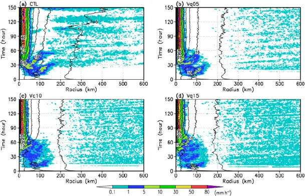
We show the time evolutions of azimuthally averaged precipitation (Fig. 3.3). Here, we regard the rainband as the precipitation system related to the eyewall within a 300 km radius from the TC center. Eyewall convection occurs near a 24 km radius from the TC center and a rainband outwardly propagating after 60 hr in CTL. The radius of 5 m s−1 tangential wind at 10 m height
increases gradually with the progress of time. The Vq experiments (Vq05, Vq10, and Vq15) show Figure 3.2: Temporal variations in maximum surface wind speed (a), area-averaged kinetic energy within a radius of 300 km from the TC center (b), and 17 m s−1 wind radius at 420 m height (c).
Results are derived from CTL (solid line), Vq05 (broken line), Vq10 (dotted line), and Vq15 (chain line). The horizontal axis shows the TC development from the initial state.
3.3. RESULTS 16
that precipitation widely spreads in the outer region of TC. That wide distribution might reflect enhanced evaporation from the sea surface because of the lower limit of the surface water vapor exchange coefficient. Nevertheless, the rainband is not readily visible. Furthermore, the strong wind radius is in a steady state depending on the lower limit. The eyewall precipitation is smaller in Vq10 and Vq15 than that in CTL. These results suggest that the eyewall more slowly develops under the influence of enhanced evaporation in the outer region.
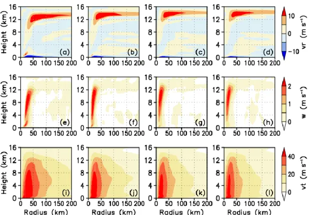
Figure 3.4 shows the radial, vertical, and tangential wind structure in the mature stage (T = 90–150 hr). In CTL, the inflow develops in the lower troposphere. The outflow has a peak value stronger than 16.0 m s−1 at around 13 km height. The vertical wind peak is located at around 25
km distance from the TC center, which corresponds well to the eyewall convection. By contrast, increasing Vq makes the eyewall and the inflow thinner and the outflow weaker than those in CTL.
The tangential wind structure becomes weaker along with increasing Vq. It is consistent with the
kinetic energy change (Fig. 3.2c).
We present the temperature anomaly (difference from average over all domains) in the inner Figure 3.3: Radius–time cross sections of azimuthally averaged precipitation (shade, mm h−1) and
surface wind speed (contour, 5 m s−1 interval) for CTL (a), Vq05 (b), Vq10 (c), and Vq15 (d). The
horizontal axis shows the distance from the TC center. The vertical axis shows the time variation from the initial state.
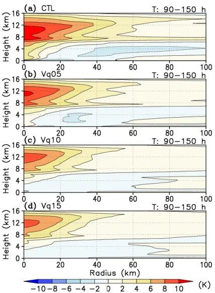
3.3. RESULTS 17
core using the difference between the inner core temperature and the area-averaged temperature (Fig. 3.5). The warm core temperature is high in CTL (+11°C) at 8–12 km height. The warm core becomes smaller and weaker with increasing Vq, which is consistent with the fact that the outflow
in the upper troposphere is weaker than that in CTL. The peak position of the temperature anomaly gradually becomes higher up to around 11–12 km with increase of the lower limit from Vq05 to Vq15. The result shows that the cloud top height becomes taller in larger Vq experiment.
Figure 3.6 shows the equivalent potential temperature (EPT) averaged over the height of 0– 100 m. In the outer region, distant from the TC center, EPT significantly and concomitantly increases with the increase of the lower limit of the surface water vapor exchange coefficient. In this region, the lower limit might strongly affect EPT in the lower troposphere. Only CTL has a negative radial gradient of near-surface EPT from the eyewall to the outer region of TC. Actually, WISHE might explain the radial gradient of EPT. In CTL, the surface water vapor exchange coefficient concomitantly decreases with increasing distance from the TC center as the wind speed Figure 3.4: Vertical structures of radial (a–d), vertical (e–h), and tangential wind speeds (i–l) averaged in the mature (T = 90–150 hr) stage for CTL (a, e, i), Vq05 (b, f, j), Vq10 (c, g, k), and Vq15 (d, h, l). Horizontal and vertical axes show distances from the TC center and altitude, respectively.
3.3. RESULTS 18
decreases. In the case of Vq05, however, the surface water vapor exchange coefficient loses wind speed dependence outside of 200 km from the TC center. Then this change suppresses the radial gradient of EPT.
Secondary circulation, which is necessary for the TC development, can be diagnosed using the mass streamfunction (Schubert and Hack 1983; Sawada and Iwasaki 2007, 2010), which is defined as
Figure 3.5: Warm core structures averaged in the mature stage (T = 90–150 hr) for CTL (a), Vq05 (b), Vq10 (c), and Vq15 (d). Horizontal and vertical axes show distances from the TC center and altitude, respectively.
3.3. RESULTS 19
𝜓 = −𝑟 ∫ 𝜌̅𝑣̅ 𝑑𝑧𝑟 𝑧 0
, (3.4)
where the overbar denotes an azimuthally averaged value and where ρ, vr, and z represent the
density, radial wind speed, and height, respectively. Figure 3.7 shows the mass streamfunction and RH. In the developing stage (T = 30–60 hr) in CTL, two positive circulations exist in the lower and middle troposphere. A high RH region exists within 30 km from the TC center in the Figure 3.6: Equivalent potential temperature (EPT) averaged in the lower troposphere (0–100 m) in the developing (T = 30–90 hr) (a) and mature (T = 90–150 hr) (b) stages. Four lines show CTL (solid), Vq05 (broken), Vq10 (dotted), and Vq15 (chain), respectively.
3.3. RESULTS 20
middle troposphere. In the mature stage, the mass streamfunction has a large value (around 4.0 × 10⁸ kg s−1) within a 600 km radius from the TC center. It is more concentrated in the lower
troposphere, indicating strong inflow near the surface. In cases with lower limits Vq, the secondary
circulation becomes weak; moreover, outer region convection causes a negative (backward) circulation in about 600 km radius from the TC center in the mature stage. It corresponds to weak inflow in the lower troposphere. The descending motion causes a low RH region at about 8 km height in both developing and mature stages.
3.4 Discussion
Results of sensitivity experiments demonstrate that introduction of the lower limit to the surface Figure 3.7: Mass streamfunction (contour, 1.0 × 10⁸ kg s−1 interval) and relative humidity
(shade, %) for four experiments in the developing (a, c, e, g) and mature (b, d, f, h) stage for CTL (a, b), Vq05 (c, d), Vq10 (e, f), and Vq15 (g, h). Mass streamfunction represents secondary circulation.
3.4. DISCUSSION 21
water vapor exchange coefficient strongly affects the TC intensity and structure. The results are not intuitive. This section includes in-depth discussion of the change in intensity and size associated with enhanced evaporation in the outer region of TC.
3.4.1 TC Intensity
Figure 3.2a suggests that enhanced evaporation in the outer region of TC suppresses intensity. According to the CISK theory (Charney and Eliassen 1964; Ooyama 1969, 1982), cumulus ensembles organized by frictional convergence near the surface release much latent heat energy of moisture and convert that energy into kinetic energy. In this sense, the water vapor content can be regarded as a fuel. However, as depicted in Fig. 3.7, convergence in the low-level inflow layer (see Fig. 3.4) becomes weak with increasing Vq in both stages: in CTL, the value of the mass
streamfunction was greater than 2.0 × 10⁸ kg s−1 within a 600 km radius from the TC center; in
contrast, in the Vq experiments, it was half of that in CTL or less. Results show that the TC intensity in CTL was markedly higher than that in the Vq experiments, although sea surface evaporation was suppressed in the outer region of TC because of weak surface winds. Therefore, the distribution of sea surface evaporation is important for TC intensification (Miyamoto and Takemi 2010; Xu and Wang 2010). Bryan and Rottuno (2009b) also showed the importance of the local radial gradient of EPT at the radius of the maximum wind for the TC intensity. Compared to the results of Xu and Wang’s (2010) experiments (OE60, OE75, OE90, and OE120), the surface water vapor exchange coefficients are altered, at least outside of 200 km from the TC center in Vq05, 100 km in Vq10, and 70 km in Vq15 in the mature stage (Fig. 3.3). It is noteworthy that the surface exchange in the eye is also altered, but as described already, the effect can be negligible. From the results of the present study, we infer that EPT outside of 200 km from the TC center can affect the TC development. As a result, the gradient of EPT between the eyewall and outside of TC is apparently more favorable than the water vapor content for the TC intensification. In fact, Figs. 3.2 and 3.6 show that the TC intensity is clearly suppressed along with the decreasing radial contrast. The conventional wind-evaporation feedback, WISHE, is constructed for the inner core region based on the positive feedback that the more water vapor content is induced by strong winds, the more TCs intensify. In this sense, the WISHE framework can be coexistent with the CISK framework. In the outer region of TC, in contrast, the present sensitivity experiments suggest that different feedback intensifies TC. This feedback consists of the process in which the weaker winds induce the less water vapor (evaporation) from the sea.
The lower limit of evaporation in the weak wind area not only suppresses the TC intensity but also delays the timing of rapid intensification. Bister and Emanuel (1997) and Bister (2001) reported that the timing of intensification is delayed if the sea surface evaporation is allowed
3.4. DISCUSSION 22
everywhere. Results suggest that the enhanced evaporation increases the lower tropospheric water vapor and that it activates cumulus convections in the outer region. That convection reduces the radial atmospheric pressure gradient in the whole troposphere and reduces the inward gradient in the lower troposphere. It is apparently unfavorable for the organization of secondary circulation of TC. The radial water vapor contrast plays an important role in TC intensification.
Figure 3.4 portrays another interesting feature of the higher outflow layer and the warm core center in the larger Vq experiment. The high total EPT in the lower troposphere in the Vq
experiments (Fig. 3.6) altered the environmental thermodynamic stability. Under the altered condition, the moist air in the eyewall might be lifted up to the higher convective neutrality level. The scenario is similar to the increase of the TC cloud top height estimated from the global Figure 3.8: Temporal variations in maximum surface wind speed (a) and area-averaged kinetic energy within a 300 km radius from the TC center (b). Results are derived from CTL (solid line), Vq01 (broken line), and Vq03 (dotted line). The horizontal axis shows the TC development from the initial state.
3.4. DISCUSSION 23
warming experiment (Yamada et al. 2010).
A phase change associated with a continuous increase of domain-integrated kinetic energy between CTL and Vq05 is apparent. In CTL, the kinetic energy grows throughout the simulation, but in Vq05, it reaches a steady state. To find the threshold, two additional experiments (Vq01 and Vq03) were conducted (Fig. 3.8). The results demonstrate that the intensity change in Vq01 (Vq03) is similar to that in CTL (Vq05), which suggests that a threshold exists between Vq01 and Vq03. The reason for the threshold remains unknown.
3.4.2 TC Size
The TC size is also important information, suggesting a disastrous area of strong winds and heavy precipitation. Furthermore, the size sometimes strongly affects the TC tracks (e.g., Iwasaki et al. 1987). The size grows with time in CTL but approaches their steady states in Vq experiments, which suggests that sea surface evaporation in the outer region of TC suppresses the size (Figs. 3.2b and 3.2c). Rainbands also influence the TC size (Hill and Lackmann 2009; Wang 2009; Sawada and Iwasaki 2010; Xu and Wang 2010). Hill and Lackmann (2009) demonstrated that the environmental RH affects the TC size through the activity of rainbands. Sawada and Iwasaki (2010) revealed that evaporation from rain drops forms rainbands and increases the TC size. Fudeyasu and Wang (2011) explained that diabatic heating in the middle–upper troposphere drives secondary circulation and forms inflow in the middle troposphere. The inflow transports the angular momentum into the outer core region and thereby develops the size. In fact, the inflow in the middle troposphere clearly forms in CTL (Fig. 3.7). The Vq experiments suggest that the dry air flows into the outer core (100–200 km radius) in the middle–upper troposphere because the dry air path is formed by the backward circulation as a result of outer region convection. The backward circulation impedes the inflow layer development and bends the secondary circulation. As a result, it suppresses the TC size.
3.5 Conclusions
We investigated the wind-evaporation feedback in the TC intensification by modification of the surface water vapor exchange coefficient in idealized cloud-resolving numerical experiments. A lower limit of the surface water vapor exchange coefficient was introduced to switch off the wind-evaporation feedback in the outer region of TC. The lower limit increases the water vapor content but reduces that radial gradient. The change attributable to the lower limit might be favorable for CISK based on moist unstable stratification. However, when increasing the lower limit of the
3.5. CONCLUSIONS 24
surface water vapor exchange coefficient, the TC intensification is slower and weaker; TC becomes smaller. The convection attributable to enhanced evaporation in the outer region suppresses the development of secondary circulation. The narrower secondary circulation inefficiently transports water vapor and angular momentum to the TC core. The lower limit of the surface water vapor exchange coefficient also suppresses the rainband activity and then reduces the TC size (Fig. 3.9). Results suggest that its radial gradient strongly controls the TC organization. The implication explained above is consistent with results of earlier works showing that deep cumulus convections in the outer region adversely affect the TC intensity (e.g., Bister and Emanuel 1997; Bister 2001; Miyamoto and Takemi 2010; Lee and Chen 2014; Sun et al. 2014; Lin et al. 2015; Rai et al. 2016). Unlike these studies, the process suggested herein is that the weaker winds induce the less water vapor (evaporation) from the sea. This feedback in the outer region of TC conflicts with the CISK framework and differs from the WISHE framework. Here, we emphasize that suppression of sea surface evaporation attributable to weak surface winds is another important aspect of the wind-evaporation feedback, which enlarges the radial gradient of Figure 3.9: Schematic diagrams of the roles of the radial contrast of water vapor mixing ratio in TCs. These diagrams show secondary circulations of TCs with (left) and without (right) the wind-evaporation process in the outer region. The orange shadings represent the water vapor mixing ratio significantly controlled by the surface evaporation. The blue shade arrows represent the strength of the secondary circulation. The circles with an inscribed X denote the TC’s tangential winds into the page and their size correspond to the wind speed).
3.5. CONCLUSIONS 25
water vapor content in the boundary layer. Figure 3.10 shows the new wind-evaporation feedback hypothesis. In the TC forecasts, particular attention should be devoted to moisture exchange in the outer region of TC. Further study should also be undertaken to elucidate wind-evaporation feedback in a realistic case.
Figure 3.10: Schematic diagram of the updated wind-evaporation feedback hypothesis. The process in which the surface light winds suppress convection outside the TC plays the role of keeping the negative gradient of water vapor (red lines).
26
Chapter 4
Case Study: TC Hagibis (2019)
4.1 Introduction
In Chapter 3, we showed the negative impacts of vigorous convection outside the TC on the intensification rate. However, these results are based on some unrealistic assumptions using the idealized simulation with horizontally uniformed environment on the f-plane, and artificial TC-like vortex. Indeed, under the realistic environmental conditions, multi-scale factors affect the TC development: the sea surface temperature (SST) distribution (Fujiwara et al. 2017, 2020a, 2020b; Hegde et al. 2016; Lee and Chen 2014; Rai et al. 2016; Sun et al. 2014), vertical wind shear, and environmental humidity (DeMaria 2009; DeMaria and Kaplan 1994; Kaplan et al. 2010, 2015; Trabing and Bell 2020; Yamaguchi et al. 2018).
To clarify the impact of the radial contrast of water vapor distribution between a TC and its outside on the intensification rate, we extract a case in which large intensity change occurred. The rapid intensification (RI) is usually defined as the 95th percentile of intensity changes over a 24-h period for t24-he western Nort24-h Pacific (WNP) TCs, and is a 30-24-hPa t24-hres24-hold over a 24-24-h period (Shimada et al. 2017). In 2019, TC Hagibis experienced a RI period in which the maximum intensification rate was −60 hPa (24 h) −1 estimated by the Japan Meteorological Agency (JMA),
or −98 hPa (24 h) −1 estimated by the Joint Typhoon Warning Center (JTWC). Figure 4.1 shows
the Hagibis’s extremely high intensification rate.
In this chapter, we examine a contribution of the inward water vapor flux and sea surface flux to the intensification process of Hagibis (2019) with two sensitivity experiments. Combining the idealized and realistic experiments, we propose a new intensification process of the wind-evaporation feedback.
4.1. INTRODUCTION 27
Figure 4.1: Intensity of TC Hagibis (2019) in terms of the maximum surface wind speed (a) and the minimum surface pressure (b) archived at JMA (black), and JTWC (red). Note that wind speed is recorded in knots (1 kt ~ 0.5144 m s−1).
4.2. EXPERIMENTAL DESIGN 28
4.2 Experimental Design
4.2.1 Model Setup
We used a nonhydrostatic model (NHM; Saito et al. 2006) to resolve small-scall phenomena in Hagibis (2019) with horizontal grid spacing of 3 km. In the terrain-following vertical direction, we set 50 atmospheric layers excluding a lower boundary layer. The topography was derived from a global digital elevation model with a horizontal grid spacing of 30 arc seconds (GTOPO30). The height of the first layer was 20 m and the top was 25 km. The vertical grid spacing was increased with height, from 40 m to 1 km. The sponge layer was inserted above 16.4 km to suppress wave reflection at the upper boundary.
We applied the Mercator map projection (Fig. 4.2), and the only vertical component of Coriolis parameter was considered without curvature terms. The buoyancy term was computed from the air density perturbation. The fourth order advection scheme was used. The time step was 12 s.
For physical processes, we used; the explicit one-moment three-ice bulk microphysics scheme (Lin et al. 1983; Saito et al. 2006) for cloud microphysics, 1.5-order turbulence kinetic energy prediction scheme (Klemp and Wilhelmson 1978; Deardorff 1980) for subgrid-scale processes, bulk coefficients with sea surface roughness prediction (Beljaars and Holtslag 1991; Kondo 1975), and no convective parameterization (Tab. 4.1).
4.2.2 Input Data
For the initial and boundary conditions, we used the 6-hourly JMA Global Spectral Model (GSM) analysis, which provided TC information. The input variables and each horizontal resolution are summarized in Tab. 4.2. The lateral boundary conditions were updated every 6 hours with relaxation damping. The integration period was from 1200 UTC on 5 October to 1200 UTC on 8 October 2019. The initial time was 6 hours prior to genesis of Hagibis and included the RI event (Fig. 4.2). The daily 0.1°-resolution SST data was derived from the high resolution merged satellite and in-situ data sea surface temperature (HIMSST).
4.2.3 Sensitivity Experiments
4.2. EXPERIMENTAL DESIGN 29
𝐹𝑞 = − max(𝑉10, 𝑉𝑞) × 𝐶𝑞(𝑞𝑣− 𝑞𝑣𝑠), (4.1)
where qv (qvs) stands for the specific humidity at the lowest atmospheric level (SST), V10
represents wind speed at a height of 10 m, and water vapor exchange coefficient was a constant,
Cq = 1.4 × 10⁻³. Unlike Chapter 3, we used one lower limit, Vq = 10 m s−1, due to two reasons.
First, since wind speeds at the lowest atmospheric level in the initial condition were under 15 m s−1 (Fig. 4.2), there was no initial local evaporation. It is unfavorable to examine the impacts of
local evaporation, WISHE. Second, we considered the boundary of the inside/outside TC to be the radius of 15 m s−1 wind speed (R15) for the future work (described in Section 4.3). We
performed two experiments: a control run applied Vq = 0 m s−1 (hereafter, CTL), and a sensitivity
experiment applied Vq = 10 m s−1 (hereafter, MIN10) (Fig. 4.3).
Figure 4.2: Track of Hagibis (2019) in the integration period (blue line; 1200 UTC 5 Oct–1200 UTC 8 Oct). The blue cross symbol indicates the Hagibis’s center observed by JMA at 1200 UTC on 5 October. The orange box represents the numerical domain. Black contour lines indicate the wind speed at the lowest model level (20-m height) at the initial time, and the hatched area denotes where its speed is larger than 10 m s−1. Shading shows the elevation from GTOPO30.
4.2. EXPERIMENTAL DESIGN 30
Table 4.1: Model settings. GSM: global spectral model, HIMSST: high resolution merged satellite and in-situ data sea surface temperature, GTOPO30: a global digital elevation model with a horizontal grid spacing of 30 arc seconds.
Table 4.2: List of GSM variables. Z: geopotential height, U: eastward wind speed, V: northward wind speed, T: temperature, RH: relative humidity, MSL: mean sea level pressure, SP: surface pressure.
4.2. EXPERIMENTAL DESIGN 31
4.3 Results and Discussion
4.3.1 Validation of Control Simulation
Here, comparing the simulated TC derived from the CTL run with the best track, we validated the reproducibility of Hagibis (2019). Figure 4.4 shows the low reproducibility of the RI onset defined as a minimum atmospheric pressure sea level decrease of a 30-hPa threshold over a 24-h period, and underestimate of the intensification rate. While the maximum rate of pressure decline derived from the CTL run was 74.7 hPa (24 h) −1 at FT = 45 hr (in the forecast time), its RI onset lagged
behind that in the best track of Hagibis (2019). The simulated TC in CTL moved northward with respect to the observed track of Hagibis (2019), and passed the relatively low SST region (Fig. 4.4). The numerical studies showed the sensitivity of locations of the TC and SST field to the simulated intensity (Lee and Chen 2014; Shamekh et al. 2020; Sun et al. 2014). According to Sun
et al. (2014), when the TC passed the vicinity of the relatively higher SST region (e.g., warm
eddies), the TC could be weakened.
To assess the synoptic fields, we referred to the 70‐year ERA starting from January 1950 onwards with timely updates (ERA5; Hersbach et al. 2020). Figure 4.6 showed the daily mean of environmental fields. Compared to the reference data, ERA5, the large-scale circulation became small and weak in lower troposphere on 6 October. Along with this, latent heat flux at the sea surface in the CTL run was smaller than that in ERA5. It decreased the radial gradient of water vapor near the surface. Because of these unfavorable conditions for the TC intensification, the RI onset was shifted behind. The compact circulation in the CTL fields were sustained on 7 October (Fig. 4.6d). The steady southern winds played in transporting water vapor into the TC center. It
4.3. RESULTS AND DISCUSSION
Figure 4.3: Schematic diagram of the disabled feedback run with a lower limit of Vq. Shading