Evaluation of an economic model composed of producer agents

Evaluation of an economic model composed of

producer agents

Nao ITOU, Yoshinobu MAEDA and Toyohiko HAYASHI

Guraduate School of Science and Technology, Niigata University

8050 Ikarashi-2, Nishi-ku, Niigata 950-2181, Japan

email:[email protected]

Abstract—In recent years, the existence of a “social divide”, comprising factors such as income and professional status, has been noted as one significant type of social issue. It has been stated that, among the disparate groups, a member belonging to one group cannot move to any other groups. Such a rigidity in terms of social status results in non-activation of the economy. In this study, we have suggested a dynamic economic model described by a multi-agent system, and have evaluated its dynamics in order to try to understand the mechanisms by which how the social divide emerges within the model. We used Gini’s coefficient to evaluate the social divide and its economic efficiency. As a result, it is suggested that economies under conditions of low competitiveness, being a state composed of relatively more consumer agents than producer agents, display a higher negative relationship between Gini’s coefficient and economic efficiency than those under conditions of high competitiveness.

I. INTRODUCTION

In recent years, the existence of a “social divide”, com-prising factors such as income and professional status, has been noted as an emerging social issue. This “divide” is defined as a difference in price, license, classification, or level and amount of information within the same class. When the income gap within a society is large, i.e., the society is in a state where ‘blue-collar’ members are not able to escape from the lowest levels in the hierarchy, then the motivation for social development will atrophy and the society will become economically dormant. In order to develop and maintain an active society, both ultra-strong and ultra-weak levels of divide are undesirable. So, is it possible to maintain an appropriate level of divide in order to encourage social development?

There are various theories as to the cause of the emergence of a social divide, such as academic background, aging of society and part-time employment. However, the mechanisms for the emergence of the social divide that are caused by the economic system are unclear. In general, a system has a tendency to generate a divide to adjust its overall efficiency. For example, multi-cellular organisms differentiate their cells into many functionally different parts to maintain the indi-vidual’s life. Similarly, an economic system is composed of characteristically different individuals.

The main purpose of this study is to investigate the relation-ship between the income divide and the economic efficiency in an economic model, and is presented in this paper using multi-agent simulation (MAS). MAS is often used when studying the dynamic features of social phenomena [1], [2].

In our economic model, the agents learn their action using reinforcement learning in order that they may be adapted to the environment.

II. MULTI-AGENTSYSTEM

A multi-agent system (MAS) is composed of many agents, and achieves a task that is difficult to achieve for a single agent or a monolithic system. In a MAS, an artificial society comprising many autonomous behavioral agents interact with each other in the simulation [1], [2]. We can contrast the phenomena simulated by a MAS with those of the real world. However, it is difficult to identify all of the relevant states because the environment in the MAS changes depending on the agent’s global features [3]. In this study, we constrain the agent to acquire an action rule, adapting it to the environment by using reinforcement learning.

III. REINFORECEMENTLEARNING

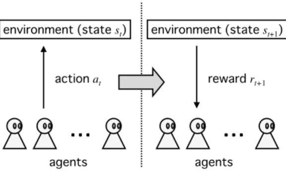
A. Definition

Reinforcement learning is a type of machine-learning that treats the problem where an agent in an environment rec-ognizes the current state, st ∈ S, and decides the action,

at ∈ A, to be taken [4]. When the agent chooses the action

at ∈ A, the state of the environment translates to st+1 ∈

S and the agent receives a reward (Fig.1). Reinforcement learning makes the agent learn the policy that offers it the maximum reward through its actions. Here the environment is formulated as a Markov decision process that has a finite number of states. Reinforcement learning is thought of as a type of ‘dynamic programming’. It is different from supervised learning, because such learning is not derived from a teacher. It has an important feature in that the agent can choose an action by developing an unknown-learning-area and an action using a known-learning-area in a balanced manner. Therefore, reinforcement learning is often used to achieve an action rules for a robot under an unknown environment. Thus, many methods of reinforcement learning have been proposed [5], [6], [7], [8], [9], [10], [11], especially in the following section, where profit sharing achieves a higher performance than alternatives when reinforcement learning is applied to the MAS’ environment [12], [13]. Therefore, we have used profit sharing in this study.

Fifth International Workshop on Computational Intelligence & Applications

agents ・・・ ・・・ ・・・ ・・・ agents ・・・ ・・・ ・・・ ・・・ environment (state st) environment (state st₊₁)

action at reward rt+₁

Fig. 1. Transition of a state in reinforcement learning.

B. Profit Sharing

Profit sharing is one type of method for reinforcement learning [12], [13]. In profit sharing, the agents are assigned a Q-value which shows the efficacy of a rule that is based on the agent’s actions, and the Q-value is updated after obtaining the reward. The rule is a pairing of the state st∈ S and the

action a ∈ A, which the agent can choose. With a state st∈ S

assigned to the environment, the agent stochastically chooses the action a ∈ A, based on policy π(st, a). We then apply the

Boltzmann choice method [14]. π(st, a) = e

Q(st,a)/T

P

a∈AeQ(st,a)/T

, (1)

where policy π(st, a) is the probability of choosing action a

in response to state st, and T is a temperature parameter. The

agent implements action a, and, as a result, the agent receives the reward rt. The Q-value, which takes the action a for state

st, is updated as follows,

Q(st, at) ← (1 − β)Q(st, at) + βrt, (2)

where β(0 ≤ β ≤ 1) represents the learning-rate.

Profit sharing is a type of non-boot-strap reinforcement learning, i.e., it does not require the next state’s Q-value when updating. Therefore, it shows a higher performance than the boot-strap method when reinforcement learning is applied to an MAS environment.

IV. PRODUCER ECONOMIC MODEL

In the mechanism of the emergence of a social divide, it is foreseen that the mechanism is included in the economic system. In this study, in order to restage the emergence of social divides as macro phenomena that are caused by the action of micro economic entities, we have structured an economic model using a MAS. In the model, we set ‘multi-merchandises’ and ‘multi-agents’. The merchandises are de-fined by the combination and permutation of two types of pri-mordial merchandise. There are three types of agent; namely the supplier agent, the producer agent and the consumer agent. A supplier agent produces unlimited primordial merchandise, and sells it. A producer agent purchases merchandise com-prising materials for his product, and he produces his product by using materials and then sells it at a price. The consumer

supplier

agents

・・

・

・・

・

・・

・

・・

・

・

・・

・

・・

・・

・

・

・・

・・

・

・・

・

・・

・

・・

・

・・・

・・・

・・・

・・・

・・・

・・・

・・・

・・・

・・

・

・・

・

・・

・

・・

・

producer

agents

consumer

agents

Fig. 2. Flow of merchandise in a producer economic model.

A

BA

AA

AB

B

BB

Fig. 3. Combination of materials and products.

agent purchases the merchandise that is finally produced by the producer agents. Fig.2 shows the flow of merchandise in a producer model. The producer agents learn appropriate action-rules concerning whether or not to purchase the material merchandise and how to price their product merchandise by reinforcement learning. The supplier agents and the consumer agents act on previously-determined action rules, i.e., not learned. In this producer economic model, we focus on the actions of the producer agents in the economic system. Here, we observe income division between the producer agents and the economic efficiency in this system, and evaluate the relationship between them.

A. Setting of merchandise

In this model, there are two types of primordial merchan-dise. We name these A and B. Merchandise AB is produced by combining A and B. In addition, merchandise BA is produced by combining A and B. Here, two kinds of merchandise can be produced by permutation. However, when the two materials are the same, such as both A and A or both B and B, only one kind of product merchandise can be produced, such as AA or BB (Fig.3). Here, we describe merchandise A and B as ‘mono-bona merchandise’, and merchandise AB, BA, AA and BB as ‘di-bona merchandise’. TABLE 1 shows the product merchandise and the combinations of the materials that constitute product merchandise up to the ‘tetra-bona level’.

B. Setting of agents

The supplier agents sell merchandise A or B at a pre-established price, pA. The consumer agents purchase

pre-TABLE I MATERIALS OF PRODUCT. Product Material Di-bona AA A+A AB A+B BA B+A BB B+B

Tri-bona AAA A+AA,AA+A AAB A+AB,AA+B ABA A+BA,AB+A ABB A+BB,AB+B BAA B+AA,BA+A BAB B+AB,BA+B BBA B+BA,BB+A BBB B+BB,BB+B Tetra-bona AAAA A+AAA,AA+AA,AAA+A

AAAB A+AAB,AA+AB,AAA+B AABA A+ABA,AA+BA,AAB+A AABB A+ABB,AA+BB,AAB+B ABAA A+BAA,AB+AA,ABA+A ABAB A+BAB,AB+AB,ABA+A ABBA A+BBA,AB+BA,ABB+A ABBB A+BBB,AB+BB,ABB+B BAAA B+AAA,BA+AA,BAA+A BAAB B+AAB,BA+AB,BAA+B BABA B+ABA,BA+BA,BAB+A BABB B+ABB,BA+BB,BAB+B BBAA B+BAA,BB+AA,BBA+A BBAB B+BAB,BB+AB,BBA+B BBBA B+BBA,BB+BA,BBB+A BBBB B+BBB,BB+BB,BBB+B

established merchandise from the producer agent who sells it at the cheapest price.

The producer agent has the following properties, M1 :Material merchandise 1．

M2 :Material merchandise 2．

P :Product merchandise．M1+ M2.

vM1 :Minimum price of material merchandise 1．

vM2 :Minimum price of material merchandise 2．

vt−1_P :Maximum price of product merchandise that was purchased on the last occasion.

s :s = (vM1+ vM2, vt−1P ). State that is recognized by

the producer agent．

a :a = (Buy, vP). Action that is chosen by producer

agent．

Buy :Variable that decides purchasing of material mer-chandise. It has values 0 or 1. When the agent does not purchase, Buy is 0. When the agent purchases, Buy is 1

vP :Sale’s price at next occasion. 0 ≤ vP ≤ 30.

C :Cost. If Buy = 0, C = 0 because the agent does not purchase anything. If Buy = 1, C = vM1+vM2.

I :Sale. If the agent’s product merchandise is pur-chased, I = vP, otherwise I = 0.

R :Income. R = I − C. It is also a reward on reinforcement learning.

Q(s, a):Q-value of state s for action a.

C. Action of agents

Step1. Each property of the agent is initialized.

Step2. An agent is selected from the producer and the consumer agents.

Step3. The selected agent recognizes the state s. The agent implements Step4 and Step5 when this agent is the producer agent, M1and M2are sold. If this agent is the producer agent and M1 and/or M2 are not sold, he does not implement Step4 and Step5, because in this case he can’t produce his product. If this agent is the consumer agent, he purchases pre-established merchandise from the producer agent who sells at the cheapest price.

Step4. The agent stochastically chooses action a based on the Q-value.

Step5. If Buy = 1, the agent purchases M1 and M2 from agents who sell them at prices of vM1 and vM2,

respectively.

Step6. All of the producers agents and the consumer agents implement Step2 to Step5.

Step7. All of the producer agents update the Q-values. Step8. All of the producer agents produce their products

using purchased material merchandises. All of the consumer agents consume his merchandise.

Step9. Reaches an end condition when the simulation ter-minates; otherwise returns to Step2.

We define the flow from Step2 to Step8 as one episode.

V. GINI’S COEFFICIENT

Gini’s coefficient (GC) is one of the barometers of social divide in economics, and has a real value between 0 and 1 [15]. When the social divide becomes larger, GC is close to 1. Assuming the presence of n ‘non-negative’ samples, y1, y2, y3, ..., yn(y1 ≤ y2 ≤ y3 ≤ ... ≤ yn), then GC is defined as GC = 1 2µyn2 n X i=1 n X j=1 |yi− yj|, (3)

where µy represents the average of yi(i = 1, 2, 3, ..., n). When

all of the samples are the same, GC = 0. GC is also defined as “The ratio of the area that is surrounded by the Lorenz curve and the line of equal share to the area of the triangle that is under the line of equal share” (Fig.4). The Lorenz curve is described by the summation of the samples to i from 1, that is, φi= i X j=1 yj. (4)

If we denote that the area that is bounded by the Lorenz curve and the line of equal share as A, the area under the Lorenz curve as B and the area of the triangle that is under

i

φ

i

(

0

,

0

)

(

n

,

0

)

(

n

,

µ

n

)

Fig. 4. Lorenz curve.

line of equal share as C, then GC is approximated as GC = A/C = (C − B)/C = 1 − B/C = 1 − n X i=1 φi/(µyn2/2) = 1 − 2 µyn2 n X i=1 φi. (5)

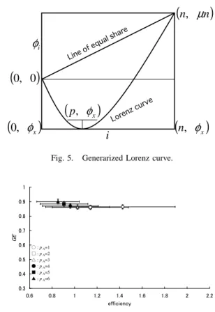
However, GC cannot be used to evaluate the divide cor-rectly when the samples include negative values. In this case, GC has the possibility of a value smaller then 0 or greater than 1. In fact, in the producer economic model considered in this study, the agent’s income may be negative. Therefore, we need to extend GC to evaluate the divide emerging in our model. Assuming n samples, y1, y2, y3, ..., yn(y1≤ y2≤ y3≤

... ≤ yn ; yi corresponds to R in section IV), and the samples

from yi to yxtake negative values. Then, the minimum of the

Lorenz curve is,

φx= x

X

i=1

yi. (6)

We redefine GC in an extended description from a geomet-ric view-point, i.e., “The ratio of the area that is surrounded by the Lorenz curve and the line of equal share to the area of a quadrangle defined by (0, 0), (0, φx), (n, φx), (n, µn)

” (Fig.5). Then, the extended Gini’s coefficient (GE) can be described as GE = 1 − 2 µyn2− 2φxn n X i=1 (φi− 2φx), (7)

where GE has a value between 0 and 1 and GE is approxi-mated as GE = n X i=1 n X j=1 |zi− zj| 2µzn2 , (8)

where zi is the linear transformation of yi following as

zi= yi−2φx n . (9) i

φ

i

(

0

,

0

)

(

n

,

φ

)

(

n

,

µ

n

)

(

0

,

φ

)

(

p

,

φ

)

Fig. 5. Generarized Lorenz curve.

0.3 0.4 0.5 0.6 0.7 0.8 0.9 1 0.6 0.8 1 1.2 1.4 1.6 1.8 2 2.2 efficiency G E ○ : pA=1 □ : pA=2 △ : pA=3 ● : pA=4 ■ : pA=5 ▲ : pA=6

Fig. 6. Relationship between economic efficiency and income divide when the number of consumer agents is 16.

µz represents the average of zi(i = 1, 2, 3, ..., n). Using yi,

GE is expressed as GE = n X i=1 n X j=1 |yi− yj| 2(µy−2φ_nx)n2 . (10) VI. SIMULATION

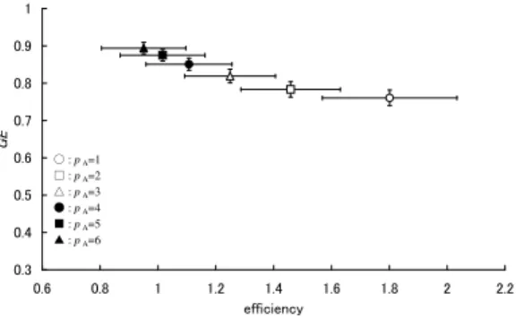
We simulated 30,000 episodes with the price of mono-bona pA set from 1 to 6. The number of di-bona producer agents, tri-bona producer agents and tetra-bona producer agents were 64, 32 and 48, respectively. We recorded the average value of GE and the average of economic efficiency from episode 20,000 to 30,000. Because the producer agent achieved suffi-cient learning, the process was terminated at episode 20,000. Economic efficiency is defined asP_NI/P_NC, where N is the number of producer agents, the learning-rate is β = 0.1, and the temperature parameter T is 1.0.

Fig. 6 , Fig. 7 and Fig. 8 corresponding to the cases in which the number of consumer agents were 16, 32, 48, respectively, show the average of GE and the economic efficiency. The abscissas and ordinates represent the economic efficiency and GE, respectively. These figures show that economic efficiency decreases with increasing price of mono-bona pA. This is because the maximum price that can be asked by the producer agent is fixed, in spite of increasing pA. The producer agents,

0.3 0.4 0.5 0.6 0.7 0.8 0.9 1 0.6 0.8 1 1.2 1.4 1.6 1.8 2 2.2 efficiency G E ○ : pA=1 □ : pA=2 △ : pA=3 ● : pA=4 ■ : pA=5 ▲ : pA=6

Fig. 7. Relationship between economic efficiency and income divide when the number of consumer agents is 32.

0.3 0.4 0.5 0.6 0.7 0.8 0.9 1 0.6 0.8 1 1.2 1.4 1.6 1.8 2 2.2 efficiency G E ○ : pA=1 □ : pA=2 △ : pA=3 ● : pA=4 ■ : pA=5 ▲ : pA=6

Fig. 8. Relationship between economic efficiency and income divides when the number of consumer agents is 48.

who produce the product made from mono-bona, can increase the price of the product. The tri-bona producer agents increase the price more. The tetra-bona producer agents can-not price above 30, which is the upper limit of the price, so the tetra-bona producer agents’ incomes decrease. Therefore, economic efficiency decreases. Economic efficiency is increased with increasing the number of consumer agents. This is because of the increased demand with increasing number of consumer agents, and the producer agents can sell their product at higher prices.

These figures show that GE increased with increasing pA. In particular, when the numbers of consumer agents is 48, GE exhibits a greater change than in the remaining cases. In the cases where the number of consumer agents are 16 and 32, numbers of the consumer agents are less than those of the tetra-bona producer agents. Therefore, a price-cutting war forces GE higher. On the other hand, when the number of consumer agents is 48, the number of consumer agents and tetra-bona producer agents are the same, so the price-cutting war does not occur. Therefore, GE depends on pA.

As a result, it is implied that economic efficiency will be reduced by increasing the price of primordial merchandise, and the income divide is increased with reducing economic efficiency. Most notably, when the number of producers and consumers are the same, i.e., when the supply and the demand are the same, the dynamic of the income divide shows an S-shaped curve for the change in the economic efficiency.

VII. CONCLUSION

In this study, we proposed a producer economic model to evaluate the relationship between economic efficiency and in-come divide. The results is suggested that for economics under conditions of low competitiveness, being a state composed of relatively more consumer agents than producer agents, display a higher negative relationship between Gini’s coefficient and the economic efficiency than those operating under high com-petitiveness. In addition, the dynamics of the income divide yields an S-shaped curve for the change in economic efficiency when the supply corresponds to the demand.

ACKNOWLEDGMENT

This research was partially supported by the Japan Society for the Promotion of Science (JSPS), Grant-in-Aid for Young Scientists (B) and the Niigata Foundation for the Promotion of Engineering.

REFERENCES

[1] Terano,T., Kita,H., Kaneda,T., Arai,K., Deguchi,H.: Agent-Based Sim-ulation -From Modeling Methodologies to Real-World Applications- ; Springer-Verlag Tokyo (2005).

[2] Adelinde M. Uhrmacher and Danny Weyns: MultiAgent Systems -Simulation and Applications- ; CRC Press Taylor & Francis Group (2009).

[3] K,Takadama: Multiagent Learning -Exploring Potentials Embedded in Interation among Agents- ; CORONA PUBLISHING CO.,LTD (2003). [4] Watkins, C.J.C.H. : Learning from Delayed Rewards; PhD thesis,

Cambridge University, Cambridge, England (1989).

[5] Sutton, R. S., Brato, A. G. : Reinforcement Learning; MIT Press, Cambridge, MA, USA, 1998.

[6] Sutton, R. S. : Learning to predict by the methods of temporal difference; Machine Learning,Vol. 3, pp.9-44, 1988.

[7] Kimura, H., Kobayashi, S. : An analysis of actor/critic algorithms using eligibility traces: Reinforcement learning with imperfect value function; In International Conference on Machine Learning, pp.278-286, 1998. [8] Konda, V. R., Tsitsiklis, J. N. : Actor-critic algorithms; SIAM Journal

on Control and Optimization, Vol.42, pp.1143-1146, 2003.

[9] Kkade, S. : A natural policy gradient; In Advances in Neural Information Processing Systems, 14, pp.1531-1538, MIT Press, 2002.

[10] Peters, J., Vijayakumar, S., Schaal, S. : Reinforcement learning for humanoid robotics; In Third IEEE/RAS International Conference on Humanoid Robots, 2003.

[11] Watkins, C. J. C. H., Dayan, P.: Technical Note: Q-Learning; Machine Learning 8, pp.279-292 (1992).

[12] Arai,S.,Miyazaki,K.,Kobayashi,S.: Methodology in Multi-Agent Rein-forcement Learning - Approaches by Q-Learning and Profit Sharing-; Technical Papers, Journal of Japanese Society for Artificial Intelligence, Vol.13, No.4, pp.609-618 (1998).

[13] Arai,S.,Miyazaki,K.,Kobayashi,S.: Cranes Control Using Multi-agent Reinforcement Learning; International Conference on Intelligent Au-tonomous System 5, pp.335-342 (1998).

[14] Sutton, R. S., Barto, A.: Reinforcement Learning; An Introduction, A Bradford Book, The MIT Press (1998).

[15] Kimura,K.: A micro-macro linkage in the measurement of inequality: another look at the Gini coefficient; Quality and Quantity 28:pp.83-97 (1994).