Ergodic control in a single product manufacturing system

(1)

Ergodic control in

a

single

product

manufacturing

system

徳大総科大橋守

(Mamoru Ohashi)

Abstract

Westudy the ergodic control problem related to stochastic production plan-ning in a single product manufacturing system with production constraints. The existence of a solution to the corresponding Bellman equation and the optimal control are shown.

1991MathematicsSubject

_{Classification.}

Primary$93\mathrm{E}20$,Secondary$93\mathrm{C}40$

.

1 Introduction

This paperdeals with the following

1d

orderdifferential equation:

$\lambda=F(\frac{\partial v}{\partial x}(x,i))-i\frac{\partial v}{\partial x}(X, i)+Av(x, i)+h(x)$, $x\in R^{1},$ $i=1,2,$

$\ldots,$

$d$

.

(1)

Here $\lambda$ is a constant, $F(x)=kx$ if

$x<0,$ $=0$ if $x\geq 0$ for

some

positive constant

$k>0,$ $h$isconvexfunction, and$A$denotes theinfinitesimal generator ofan irreducible

Markov chain $(z(t), P)$ _with statespace $Z=\{1,2, \ldots, d\}$

:

$Av(x,i)= \sum j\neq iq_{ij}[v(\mathcal{I},j)-v(_{\mathcal{I}},i)]$, (2)

where $q_{ij}$ is thejump rate of$z(t)$ from$i$ to$j$. Theunknown

are

thepair $(v, \lambda)$, where

$v(\cdot,i)\in C^{1}(R^{1})$ for

every

_{$i\in Z$}.

Equation (1) arises in theergodic control problem ofstochastic production

plan-ning in a single product

manufacturing

system and is called the Bellman equation. The inventory level $x(T)$ of stochastic production planning modeled by Sethi _and

Zhang [11] is govemed by the differentialequation

(2)

for production rate $0\leq p(t)\leq k$, in which $z(t)$ is interpreted as the demand rate.

For ergodic control, the cost $J(p(\cdot) : x, i)$ associated with $p(\cdot)$ is given by

$J(p( \cdot) : x, i)=\lim_{T-}\sup_{\infty}\frac{1}{T}E[\int_{0}\tau_{h(x(t))dt}|x(\mathrm{O})=X, Z(\mathrm{O})=i]$, (4)

where $h(x)$ representsthe convex inventory cost.

Thepurpose ofthis paperis to show the existenceofasolution ofBellman

equa-tion (1) and to present an optimal control minimizing the cost $J(p(\cdot) : x, i)$ subject

to (3). In the control problem ofmanufacturing systems [5], [12] with discounted rate

$\alpha>0$, many authors have investigated the Bellmanequation

$\alpha u_{\alpha}(x, i)=F(\frac{\partial u_{\alpha}}{\partial x}(x, i))-i\frac{\partial u_{\alpha}}{\partial x}(X,i)+Au_{\alpha}(x, i)+h(x)$. (5)

Our

method consists in studying the limit of (5) as $\alpha$ tends to $0$. This approach

developsthe techniqueofBensoussan-Frehse [2] concerning non-degenerate$2^{nd}$ order

partial differential equations to our degenerate case. We also refer to Ghosh et al.

[7], [8] in the case that the Brownian motion is added to (3) as sales returns and a

bounded restriction on production rate$p$ is made.

Section 2 is devotedto the existenceproblem of (1) under the convexity

assump-tion and others on $h$, and properties of the solution are shown in

\S

3. In

\S

4 an

optimal control for the ergodic control problem and the value are given. In

_\S

5

we

present anexample of the solution to (1).

2 Existence

We are concerned with the equation

$\alpha u_{\alpha}(x,i)=F(\frac{\partial u_{\alpha}}{\partial x}(x,i))-i\frac{\partial u_{\alpha}}{\partial x}(X,i)+Au_{\alpha}(x, i)+h(x)$ _{$x\in R^{1},$} _{$i\in Z$}, (6)

and make the following assumptions:

$h(x)$ is nonnegative and convex on $R^{1}$, (7)

$\exists C>0;0\leq h(x)\leq C(1+|x|^{\kappa})$ for some positiveinteger $\kappa$, (8)

$k$

.

$-d>0$

. (9)

Theorem 2. 1 We assume (7), (8) and (9). Then there enists a unique convex

solution$u_{a}(\cdot,i)\in C^{1}(R^{1}),$$i\in Z$

of

equation (6) such fhat

$\alpha||u_{\alpha}(\cdot,i)||_{L(I)}\infty r\leq K_{r},$, (10)

$|| \frac{\partial u_{\alpha}}{\partial x}(\cdot,i)||L\infty(I_{\mathrm{r}})\leq K_{r}$, (11)

(3)

where $K_{r}$ is a positive constant depending only on $r$

of

$I_{r}=(-r,r)$.

Proof. According to [11, Theorem 3.1], equation (6) has a viscositysolution [6] given

by

$u_{\alpha}(x,i)= \inf_{p(\cdot)\in p(x,i)}\{E[\int^{\infty}\mathrm{o}e^{-}\alpha\# h(x(t))dt|x(\mathrm{o})=x, Z(\mathrm{O})=i]\}$,

where $x(t)$ is as in (3), and the infimum is taken over the class $P(x, i)$ of control

processes $p(\cdot)$ such that $0\leq p(t)\leq k$ and $p(t)$ is adapted to $\mathcal{F}_{t}=\sigma(z(s),S\leq t)$

.

Moreover, $u_{\alpha}(x, i)$isconvexandhencea classicalsolutionof(6) in$C^{1}(R^{1})$

.

As is

well-known [9], for theirreducible Markov chain $(z(t), P)$ thereexists a unique equilibrium

distribution $\pi=(\pi_{1}, \pi_{2}, \cdots, \pi_{d})>0$ such that

$\pi A=0$ _and

$\sum_{i\in Z}\pi_{i}=1$. (13)

Now, multiplying (6) by $\pi_{i}$ and summing up, we have

$\alpha\sum_{i}\pi_{i}u_{\alpha}(X,i)=\sum_{i}\pi_{i}\{F(\frac{\partial u_{\alpha}}{\partial x}(X, i))-i\frac{\partial u_{\alpha}}{\partial x}(X,i)\}+h(X)$. (14)

Since $F(x)-i_{X}\leq 0$ under (9), we have

$\alpha\sum_{*}\pi_{i}u_{\alpha}(_{X}, i)$

$\leq$ $h(x)$

$\leq$ $K_{r}$ on $I_{r}$

.

Thus we can obtain (10) by$u_{\alpha}(x, i)\geq 0$.

Next, note that

$F(x)-i_{X}\leq-a|x|$, ₍₁₅₎

where $a= \min\{k-d, 1\}>0$. Hence, we have by (14)

$a \sum_{i}\pi_{i}|\frac{\partial u_{\alpha}}{\partial x}(_{X},i)|\leq h(x)-\alpha\sum_{i}\pi_{i}u_{a}(X, i)$

.

Thus we deduce $| \frac{\partial u_{\alpha}}{\partial x}(x, i)|\leq K_{r}$ on $I_{r}$ by (10) and then (11). Finally, (12) follows

from (6), (10) and (11) immediately.

Next we show the behavior ofasolution to equation(6) as $\alphaarrow 0$.

Theorem 2. 2 Under the assumptions

_of

Theorem 2. 1

,

there exists a $\mathit{8}ub_{Seq}uence$

$\alphaarrow \mathit{0}$ such that

$v_{\alpha}(x,i)$ $:=$ $u_{\alpha}(x,i)-u(\alpha \mathrm{O},i)$ $arrow$ $v_{0}(X,i)\in C^{1}(R^{1})$,

(4)

unifomdy on each$\overline{I}_{r}$. The limit

$(v_{0}(\cdot, i),\mu i),$ $i\in Z$,

satisfies

$\mu_{i}=F(\frac{\partial v_{0}}{\partial x}(x,i))-i\frac{\partial_{U_{0}}}{\partial x}(X,i)+Av_{0}(x,i)+h(x)$, $x\in R^{1}$

.

(16)

Proof. Let us notethat $(v_{\alpha}(\cdot,i),\mu(\alpha))$ satisfies

$\alpha v_{a}(x,i)+\mu(\alpha)=F(\frac{\partial_{U_{\alpha}}}{\partial x}(x, i))-i\frac{\partial v_{a}}{\partial x}(X, i)+Av_{\alpha}(x,i)+h(x)$

.

(17)

By (11) it is obvious that

$||v_{\alpha}( \cdot,i)||_{L^{\infty}(I_{\mathrm{r}}})+||\frac{\partial v_{\alpha}}{\partial x}(\cdot, i)||L\infty \mathrm{t}I_{\gamma})\leq K’$

’ $i\in Z$

.

(18)

Hence $\{v_{a}(\cdot, i)\}$ is equicontinuous

on

$\overline{I_{l}}.$

.

Let

us

define

$B_{\alpha}(x)=\alpha v\alpha(x,i)+\mu(\alpha)-Av(\alpha x,i)-h(x)$

.

We recall that, by assumption, $h(x)$ is Lipschitz continuous on $\overline{I_{l}}.$. Then,

by (18)

$|B_{\alpha}(X)-B_{\alpha}(y)|\leq C|x-y|$, ($C>0$ : indep. of$\alpha$),

From (17) it follows that

$B_{\alpha}(x)=F( \frac{\partial v_{a}}{\partial x}(x,i))-i\frac{\partial v_{\alpha}}{\partial x}(x, i)$,

Then

we

have

$\frac{\partial v_{\alpha}}{\partial x}=\{$

$\frac{B_{\alpha}\langle x)}{k-i}$ if $\frac{\partial v_{\alpha}}{\partial x}<0$

$- \frac{B_{\alpha}(x)}{i}$ if $\frac{\partial v_{\alpha}}{\partial x}\geq 0$,

Since $\frac{\partial v_{\alpha}}{\partial x}$ is nondecreasing, we

can

see

$| \frac{\partial v_{\alpha}}{\partial x}(_{X,i})-\frac{\partial v_{\alpha}}{\partial x}(y, i)|\leq C|x-y|$.

Thus $\{\frac{\partial v_{\alpha}}{\partial x}$(.,$i$)$\}$ is also equicontinuous on $\overline{I}_{r}$

.

By the Ascoli-Arzel\‘a _{theorem, there}

exists a subsequence $\alphaarrow 0$ such that

$v_{\alpha}(X,i)$ _{$arrow v_{0}(X,i)$},

(19)

$\frac{\partial v_{\alpha}}{\partial x}(x,i)$

$arrow$ $\frac{\partial v_{0}}{\partial x}(x, i)$,

uniformly

on $\overline{I}_{r}$

.

(20)

By a standardargument, we can choose a subsequence$\alphaarrow 0$, independent of

$r$, such

that (19) and (20) are

fulfilled on every

$\overline{I}_{r}$.

Further, by (10) and (12)

$\mu(\alpha)$ $arrow$ $\mu_{i}$

.

Letting

$\alphaarrow 0$ in (17), we deduce (16). The

proof is complete.

(5)

$\mathrm{T},\mathrm{h}\mathrm{e}\mathrm{o}\mathrm{r}\mathrm{e}\mathrm{m}2.3$ We

assume

(7), (8) and (9). Then there exists a solution

$(v, \lambda)$

of

equation (1) such that$v(x, i)$ is convex on$R^{1}$ and_{$v(\cdot, i)\in C^{1}(R^{1})$}

.

Proof. Let us define

$v(x,i)=v_{0}(X,i)+f(i)$,

$\lambda=\sum_{i}\pi_{i}\mu i$,

where $(v_{0}(., i),\mu_{i})$ is

as

in (16) and $f(i)$ is

a

solution of

$Af(i)=-\mu i+\lambda,$ $i\in Z$

.

(21)

Then it is easily seen that $(v, \lambda)$ satisfies (1). The convexity of$v(x, i)$ and $v(\cdot,i)\in$

$C^{1}(R^{1})$ are$\mathrm{i}\mathrm{m}\mathrm{m}\epsilon A$iate from Theorems 2.1 and2.2.

To complete the proof, it is sufficient to check the existence of $f(i)$

.

By the

irreducible Markov chain $(z(t), P)$ it follows that for

any

$g\in R^{d}$ $E[g(z(s/ \alpha))]arrow\sum_{i}\pi_{i}g(i)$ as $\alphaarrow 0$

.

Hence

$\alpha G_{\alpha}g(i)$ $=$ $\alpha E[\int_{0}^{\infty}e^{-}g(\alpha lZ(t))dt]$

$=$ $\int_{0}^{\infty}e^{-s}E[g(z(_{S/}\alpha))]d_{S}$ $arrow$

$\sum_{\dot{l}}\pi_{i}g(i)=\pi g$,

where $G_{\alpha}$ denotes the resolvent operator ofthe Markov chain $(z(t), P)$

. According

to [4, Lemma $7.3(\mathrm{c},\mathrm{d})$, p.39], we can obtain the relation:

$\{g\in R^{d}|\pi g=0\}=\{Ag\in Rd|g\in Rd\}$

.

We notice by (13) that

$\pi(-\mu$_. $+\lambda)=0$

.

Therefore we conclude that equation (21) admits asolution $f(i)$

.

3 Properties

Weinvestigate properties ofasolutiontothe Bellman equation (1). Nowwemake

the assumption:

(6)

Lemma 3. 1 Under (22), the

convex

solution $v(\cdot,i)\in C^{1}(R^{1})$

of

equation (1)

sat-isfies

$| \frac{\partial v}{\partial x}(x, i)|$ _$arrow$ $\infty$ as $|x|arrow\infty$

.

(23)

Proof. It is sufficient to show (23) in the case$xarrow-\infty$. By the convexity of$v(x,i)$,

we can define $M_{i}$ by

$M_{i}=-x arrow\lim_{-\infty}\frac{\partial v}{\partial x}(_{X,i})$.

For

any

sequence $x_{n}arrow-\infty$,

we

can easily see

$\frac{v(x_{n},i)}{|x_{n}|}$ $arrow$ $M_{i}$.

Suppose that $M_{i}<\infty$ for

some

$i\in Z$. Then, dividing (1) by $|x_{n}|$ and passing to the

limit, wehave by (22)

$\lambda/|x_{n}|=[F(\frac{\partial v}{\partial x}(Xn’ i))-i\frac{\partial v}{\partial x}(_{X_{n},i})+\sum_{\neq ji}q_{i}jv(x_{n},j)$

$- \sum_{j\neq i}q_{i}jv(_{X}n’ i)+h(X)n]/|x_{n}|$ $arrow\infty$,

since $v(x,j)\geq ax+b$ for some constants $a$ and $b$

.

This is a contradiction. Hence

$M_{i}=\infty$ for all $i\in Z$, and thus the assertionfollows.

Lemma 3. 2 For the convex solution $v(\cdot,i)\in C^{1}(R^{1})$

of

equation (1), there is a

constant$C>0$ such that

$|v(x,i)|\leq C(1+|x|^{\kappa+1})$. ₍₂₄₎

Proof. From (1) and (15) it followsthat

$\lambda\leq-a|\frac{\partial v}{\partial x}(x, i)|+Av(x, i)+h(x)$.

If $\frac{\partial v}{\partial x}(x, i)<0$ on someinterval _{$(-\infty, x_{1})$} with

$x_{1}<0$, then by (8)

$- \frac{\partial v}{\partial x}(x, i)\leq\frac{1}{a}Av(x,i)+C(1+|x|^{\kappa})$ ₍₂₅₎

Multiplying (25) by $\pi_{i}$ and summing up,

we

get by (13)

(7)

Integrating

over

$(x,x_{1})$, wehave

$\sum_{1}\pi_{i}(v(X,i)-v(X1,i))\leq c(1+|_{X|}k+1)-$

.

This relation can be obtained in thecase that $\frac{\partial v}{\partial x}\geq 0$

on some

interval $(x_{2}, \infty)$ with

$x_{2}>0$

.

Therefore we can obtain the desired result by $\pi>0$.

Next, we consider the equation

$\frac{d_{X^{*}}(t)}{dt}=p^{*}(x(*t), Z(t))-z(t),$ $x^{*}(\mathrm{O})=x$, $z(\mathrm{O})=i$, P-a.s., (26)

where

$p^{*}(x, i)=\{$

$k$ if $\frac{\partial v}{\partial x}(x,i)<0$ $i$ if $\frac{\partial v}{\partial x}(x,i)=0$

$0$ if $\frac{\partial v}{\partial x}(x,i)>0$.

(27)

Lemma 3. 3 Equation $(\mathit{2}\theta)admit\mathit{8}$a unique solution $x^{*}(t)$, which

satisfies

$\sup_{t}||X^{*}(t)|.|_{L}\infty<\infty$

.

Proof. Since$p^{*}(x, i)$ is nonincreasing in$x$, the differential equation (26) hasaunique

solution by [6, Theorem 6.2].

To complete the proof, let $\overline{x}=\sup$

{

$x\in R^{1}$

:

$p^{*}(x,i)\geq i$ for some $i\in Z$

}.

Obviously, $\overline{x}$ is finite, because$p^{*}(x, i)$ is nonnegative. Similarly, let $\tilde{x}=\inf\{x\in R^{1}$

:

$p^{*}(x, i)\leq i$ for some $i\in Z$

}.

Supposethat $\tilde{x}$isnot finite. Then thereexists$i\in \mathrm{Z}$ such

that $\frac{\partial v}{\partial x}(X, i)\geq-2i$ forall$x\in R^{1}$. Onthe other hand, by Lemma 3.1, $\frac{\partial v}{\partial x}(x, i)arrow-\infty$

as $xarrow-\infty$. This is acontradiction.

Now, if $x^{*}(t)>\overline{x}$ (resp. $x^{*}(t)<\tilde{x}$), then $\frac{dx^{*}}{dt}(t)<0$ (resp. $\frac{dx^{*}}{dt}(t)>0$). Hence

the interval $[\tilde{x},\overline{x}]$ is an attracting set for (26). Thus the $\mathrm{b}\mathrm{o}\mathrm{u}\mathrm{n}\mathrm{d}\mathrm{e}\mathrm{d}\mathrm{n}\in \mathfrak{B}\mathrm{S}$ of _$x^{*}(t)$ is

immediate.

Lemma 3. 4 The constant solution $\lambda$

of

equation (1)

_satisfies

$\lambda=\inf_{xp(\cdot)\in P(i)},\lim_{\alphaarrow}\sup_{0}\alpha E[I_{0}\infty xe^{-}((\alpha_{h}tt))dt|x(\mathrm{O})=x, z(\mathrm{O})=i]$ . (28)

Proof. For the

convex

solution$v(\cdot, i)\in C^{1}(R^{1})$, let us apply an elementary rule and

Dynkin’s formula to the first and the second variables of $v(x(t), z(t))$ respectively.

Then wehave the relation:

$E[e^{-\alpha t}v(x(t), z(t))|x(\mathrm{O})=x, z(\mathrm{O})=i]$

$=v(x,i)- \alpha E[\int^{t}0)e^{-}\alpha sv(x(S), z(s)dS|x(\mathrm{O})=x, z(\mathrm{O})=i]$

$+E[I_{0}^{t}e^{-\alpha} \frac{\partial v}{\partial x}S(X(S), Z(S))dX(s)|x(\mathrm{O})=x, z(\mathrm{O})=i]$ (29)

(8)

We notice that the minimumof

$\min_{0\leq P\leq k}p\frac{\partial v}{\partial x}=F(\frac{\partial v}{\partial x})$

is attained by$p^{*}(X, i)$

.

By (1), we have

$\lambda\leq\frac{\partial v}{\partial x}(x,i)(p-i)+Av(x,i)+h(x)$, (30)

and theequality holdsfor $p=p^{*}(x,i)$. Clearly, by (3)

$|X(t)|\leq C(t+1)$ for all $p(\cdot)\in P(x, i)$.

By Lemma

3.2

$E[e^{-\alpha t}|v(X(t), z(t))||x(\mathrm{O})=x, z(\mathrm{O})=i]$

$\leq CE[e^{-\alpha}(t1+|x(t)|^{\kappa+}1)|x(\mathrm{O})=x, z(\mathrm{O})=i]$

$\leq Ce^{-\alpha}(t1+(t+1)^{\kappa+1})arrow 0$ as $tarrow\infty$

.

Hence, substituting (30) into (29),

we

get

$\lambda$

$\alpha$

$\leq$ $-v(X,i)+ \alpha E[\int^{\infty}0(e-\alpha sv(_{X}(s), zs))ds|x(0)=X, Z(0)=i]$

$+E[ \int_{0}\infty e-\alpha sh(x(S))dS|x(\mathrm{O})=x, z(\mathrm{O})=i]$

.

We note that by Lemma 3.2 and 3.3

$\alpha^{2}E[\int_{0}^{\infty}e^{-}|v(x(s), z(aSs))|d_{S}|x(0)=x, Z(0)=i]$

$\leq\alpha^{2}C\int_{0}^{\infty}e-\alpha s(1+|x^{*}(S)|\kappa+1)dsarrow 0$

as

$\alphaarrow 0$

.

Thus we deduce

$\lambda\leq\inf_{Pp(\cdot)\in(x,i)}\lim_{\alphaarrow 0}\sup\alpha E[\int 0h\infty e^{-}\alpha S(X(_{S}))d_{S}|x(0)=X, z(0)=i]$,

and the equalityholds for$p(t)=p^{*}(x^{*}(t), z(t))$ of (27).

4 An

application

to

ergodic

control

We _{shall study the ergodic control problem to} $\dot{\mathrm{m}}\mathrm{m}$imize the cost:

(9)

over all$p(\cdot)\in U$ subject to

$\frac{dx(t)}{dt}=p(t)-z(t)$, $x(0)=x,$ $z(\mathrm{O})=i$, P-a.s.,

where $U$ is the set of all nonnegative progressively

measurable processes

$p(t)$ such

that

$p(t)$ is adapted to$\mathcal{F}_{t}$, $0\leq p(t)\leq k$,

$\sup_{t}E[|X(t)|^{\kappa+1}|x(0)=x, Z(\mathrm{o})=i]<\infty$ for $\kappa$ in (8).

Theorem 4. 1 We

assume

(7), (8), (9) and (22). Then ffie optimal control$p^{*}(t)$ is

given by

$p^{*}(t)=p*(x*(t), z(t))$, $atd$ ffie value by

$J(p^{*}(\cdot) : x,i)=\lambda$,

where$p^{*}(x^{*}(t), z(t))$ is as in (27).

Proof. From thesame formula as (29) it follows that

$E[v(X(\tau),\mathcal{Z}(T))|x(\mathrm{O})=x, z(\mathrm{o})=i]$

$=v(x,i)+E[ \int_{0}^{T}\frac{\partial v}{\partial x}(x(\mathit{8}), z(S))dx(s)|x(\mathrm{O})=x, z(\mathrm{o})=i]$

$+E[ \int_{0}T(Av(x(s), Zs))dS|x(\mathrm{O})=x,z(\mathrm{o})=i]$.

We recall (30) to obtain

$E[v(X(\tau), Z(T))|x(\mathrm{O})=X, Z(\mathrm{O})=i]$

$\geq v(x, i)+E[\int_{0}^{\tau}(\lambda-h(x(s)))ds|x(\mathrm{O})=x, z(\mathrm{o})=i]$ ,

where the equality holds for $x=x^{*}$ and $p=p^{*}of(27)$

.

By Lemma 3. 2 and the

definition of$U$

$\frac{1}{T}E[|v(x(\tau), \mathcal{Z}(T))||x(\mathrm{O})=x, z(\mathrm{O})=i]$

$\leq\frac{C}{T}E[1+|x(\tau)|^{k+1}|x(\mathrm{O})=x, z(\mathrm{O})=i]$ $arrow$ $0$ as $Tarrow\infty$.

Also, by Lemma3. 3 , $p^{*}(t)$ belongs to $U$. Thus wededuce

$J(p(\cdot) : x,i)$ $=$ $\lim_{Tarrow}\sup_{\infty}\frac{1}{T}E[I_{0}\tau)h(X(S)d_{S}|x(\mathrm{O})=x,z(\mathrm{O})=i]$

$\geq$ $\lambda=J(p^{*}(\cdot):X,i)$

.

(10)

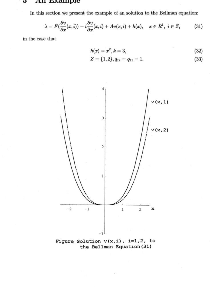
5 An Example

In this section we present the exampleofan solution to the Bellman equation:

$\lambda=F(\frac{\partial v}{\partial x}(x,i))-i\frac{\partial v}{\partial x}(X,i)+Av(x, i)+h(x)$, $x\in R^{1},$ $i\in Z$, (31)

in thecase that

$h(x)=x^{2},$$k=3$, (32)

$Z=\{1,2\},$$q_{1}2=\infty 1=1$. (33)

Figure Solution v(x, i)

,

$\mathrm{i}=1$,2, to

(11)

We remark that the matrix induced by $A$ is given by

$A=$

,

and the equilibrium distribution$\pi$ is

$\pi=$

.

Thereforethe assumptions ofTheorem 4.1 are fulfilled.

Now, recalling the form ofoptimal control $p^{*}$ and solving the Bellman equation

(31) with (32) and (33), we have

$\lambda=0$, $v(x, 1)=\{$ $\frac{1}{81}(18x^{3}+18x^{2}-24x+16-16e^{-\frac{3}{2}x})$ if $x\geq 0$ $- \frac{1}{81}(18x^{3}+9x^{2}+12x+8-8e^{\frac{3}{2}x})$ if$x<0$, $v(x,2)=\{$ $\frac{1}{81}(18x^{3}-9x2+12x-8+8e^{-\frac{3}{2}x})$ if$x\geq 0$ $- \frac{1}{81}(18x^{3}-18X-224x-16+16e^{\frac{3}{2}x})$ if$x<0$

.

Then the optimal control$p^{*}$ is given by

$p^{*}(x,i)=\{$

$0$ if $x>0$

$i$ if $x=0$

3

if $x<0$.

The solution $v(x, i)$ with (23) $-(24),$ $\mathrm{i}=1,2$ can be shown in Figure.

References

[1] A. Bensoussan, S.P. Sethi, R. Vickson and N. Derzko, Stochastic production

planning with production constraints, SIAM J. Control and Optim., 22 (1984),

pp. 920-935.

[2] A. Bensoussan and J. Frehse, On Bellman equations of ergodic control in $R^{n}$,

J. reine angew. Math.,

429

(1992), pp. 125-160.

[3] E.B. Dynkin, Markov Processes, vols.I,II, Springer-Verlag, Berlin, 1965.

[4] S.N. Ethier and T.G. Kurtz, Markov Processes: Characterization and

Conver-gence, John Wiley&Sons, New York, 1986.

[5] W.H. Fleming, S.P. Sethi and H.M. Soner, An optimal stochastic production

planning problem with randomly fluctuating demand, SIAM J. Control and

(12)

[6] W.H. Fleming and H.M. Soner,

Controlled

Markov Processes and Viscosity

Solutions, Springer-Verlag, Berlin,

1993.

[7] M.K. Ghosh, A. Arapostathis and S.I. Marcus, Optimal control of switching

diffusions with application to flexible manufacturing systems, SIAM J. Control

and Optim.,

31

(1993), pp.

11831204.

[8] M.K. Ghosh, A. Arapostathis and

S.I.

Marcus, Optimal control of a hybrid system with pathwise average cost, Proceedings ofthe

31st

CDC, (1992), pp.

1061-1066.

[9] P. Hartman, Ordinary Differential Equations,

Birkh\"auser,

Boston, 1982.

[10] J. Lamperti, Stochastic Processes, Appl. Math.

Sci.

23,

Springer-Verlag,

Berlin,

1977.

[11] S.P. Sethi and Q. Zhang, Hierarchical Decision Making in Stochastic Manufac-turing Systems,

Birkh\"auser,

Boston,

1994.

[12] S.P. Sethi, H.M. Soner, Q. Zhang and J. Jiang, Tumpike Sets and their Anal-ysis in Stochastic Production Planning Problems, Mathematics of Operations