Computing the Combinatorial Canonical Form of a Layered Mixed Matrix

(1)

Computing

the

Combinatorial Canonical

Form

of

a

Layered Mixed

Matrix

京大数理研室田–雄(Kazuo Murota, Kyoto U)

ミュンヘン工科大マーク

.

シャープロ$-$ ト (Mark Scharbrodt, $\mathrm{T}\mathrm{U}-\mathrm{M}\ddot{\mathrm{u}}\mathrm{n}\mathbb{C}\mathrm{h}\mathrm{e}\mathrm{n}$)

1. Introduction. A matrix

$A=$

is said to be layered mixed (or $\mathrm{a}.\mathrm{n}$

LM-matrix), if the set of

nonzero

entries of $T$ is algebraically independent

over

the field to

which the entries of $Q$ belong. Its Combinato$r\cdot ial$ Canonical Form ($CCF$ for short) is

a

(combinatorially unique) finest block-triangular representation of the matrix under the ad-missible $\mathrm{t}\mathrm{r}\mathrm{a}\mathrm{n}\mathrm{S}\mathrm{f}\mathrm{o}\mathrm{r}\mathrm{m}\mathrm{a}\mathrm{t}\mathrm{i}_{\mathrm{o}\mathrm{n}}$

. of the form

$P_{r}P_{c}$

,

where $S$isanonsingularmatrix,and$P_{r}$ and $P_{c}$

are

permutation matrices. Inthe CCF, each

diagonal block is afull rank square matrix. For a singular or rectangular matrix the CCF

includes also full rank horizontal $\mathrm{a}\mathrm{n}\mathrm{d}/\mathrm{o}\mathrm{r}$ vertical tails. Note that the CCF reduces to the

well-known Dulmage-Mendelsohn decomposition [BR91, DER86, DM59, DR78, EGLPS87,

Gu76, Ho76, PF90] if the $Q$-part isempty.

Example 1. If $t_{i}(i=1,2,3,4)$ denote independent parameters, $A$ below is a $4\cross 5$

$\mathrm{L}\mathrm{M}$-matrix, andits CCF is given by

$\tilde{A}$, which consists ofa _{$1\cross 2$} horizontal tail and a_{$3\cross 3$}

square nonsingular block, with an emptyvertical tail:

$A==$

,

$\tilde{A}=$

.

The conceptof mixed matriceswasintroducedbyMurota-Iri [MI85] as atoolfor describ-ingdiscrete $\mathrm{p}\mathrm{h}\mathrm{y}\mathrm{s}\mathrm{i}\mathrm{c}\mathrm{a}\mathrm{l}/\mathrm{e}\mathrm{n}\mathrm{g}\mathrm{i}\mathrm{n}\mathrm{e}\mathrm{e}\mathrm{r}\mathrm{i}\mathrm{n}\mathrm{g}$systems (see [Mu96] forexposition), and subsequently, the

CCFof$\mathrm{L}\mathrm{M}$-matriceswasestablished by$\mathrm{M}\mathrm{u}\mathrm{r}\mathrm{o}\mathrm{t}\mathrm{a}-\mathrm{I}\mathrm{r}\mathrm{i}$-Nakamura [MIN87] and Murota [Mu87].

An efficient algorithm for computing the CCF was designed with matroid theoretical meth-ods (submodularflow model). This algorithm, to be described in Section 2, operates in two phases; the first phase detects a maximal independent assignment in an auxiliary network,

and the second phase finds the decomposition.

In the present paper, we deal with practical computing of the CCF. Since engineering

applications usually are large scale, it is important to identify typical characteristics in practical situations in orderto significantly speed up the algorithmon top of its theoretical

efficiency. In that line, based on the original algorithm, we will present practically faster versions which

use

simple but very effective procedures in order to improve solving the underlying independent assignmentsubproblem. Also, wediscuss implementationstrategies. We implemented the algorithm in the Mathematicalanguagewhich is suitableespeciallyfor symbolic computation. The code is available viaanonymousftp (seeAppendix Afordetails). 2. The original CCF-algorithm. The CCF ofalayered mixed matrix canbe

com-puted by first identifying

a

maximum independent assignment in

an

associated bipartite

graph, and then applying the ${\rm Min}-\mathrm{c}_{\mathrm{u}}\mathrm{t}-\mathrm{d}\mathrm{e}\mathrm{c}\mathrm{o}\mathrm{m}\mathrm{P}\mathrm{o}\mathrm{S}\mathrm{i}\mathrm{t}\mathrm{i}\mathrm{o}\mathrm{n}$ to the resulting auxiliary network.

This is based on the fact that the rank of alayered mixed matrix can be characterized by

the minimum value of a certain submodular function that can be represented as the cut function ofanindependent assignment problem. In what follows,wedescribe the algorithm of [Mu93], while referring the reader to $[\mathrm{M}\mathrm{u}87][\mathrm{M}\mathrm{u}93]$ fortheoretical backgrounds.

For alayered mixed matrix $A$, we define $R_{T}=\mathrm{R}\mathrm{o}\mathrm{w}(\tau)$ and $C=\mathrm{C}\mathrm{o}1(A)$

.

Furthermore,

(2)

networkfor the underlying independent assignment problem is

a

directed graph$G=(V,B)$

with vertex set $V=R_{T}\cup C_{Q}\cup C$ and

arc

set $B=B_{T}\cup B_{C}\cup B^{+}\cup M$, where $B_{T}=$

$\{(i,j)|i\in R_{T}, i\in C, T_{ij}\neq 0\},$ $B_{C}=\{(j_{Q},j)|j\in C\}$ and $B^{+}$ and $M$

are arcs

which

are

dynamically defined with respect to the current independent assignment; $B^{+}$ allows to

perform exchanges in the base of matrix $Q$, whereas $M$ is built by the reversals of the

arcs

matched in the assignment. We denote by$\partial M$ the set of end vertices of_$M$

.

In addition, the algorithm works on two matrices $P$ and $S$ and a vector base. At the

beginning of the algorithm, $P$ is set to $Q$ and finally, after executing pivotings, $P$

can

be

permuted to a block triangular matrix according to the CCF decomposition. The other matrix $S$

gi.ves

the matrix $S$in the admissibletransformation. The variable base is

a

vector

of size$m_{Q}$, which represents

a

mapping $R_{Q}arrow C\cup\{0\}$

.

Then,the algorithm

can

be stated asfollows, where Step 1 to Step 3 computetheindependent assignment and Step 4aims at processing the decomposition:

[Algorithm for the CCF of a layered mixed matrix $\mathrm{A}$]

Step 1: $M:=0;base[i]:=0(i\in R_{Q});P[i,j1:=Q_{1j}.(i\in R_{Q}, j\in C)$;

$S:=\mathrm{u}\mathrm{n}\mathrm{i}\mathrm{t}$ matrix of order

$m_{Q}$

.

Step 2: $I:=\{i\in C|i_{Q}\in\partial M\cap C_{Q}\}$;

$J$ _{$:–\{j\in C-I|\forall i:base[i]=0\Rightarrow P[i,j]=0\}$};

$S_{T}^{+}:=R\tau-\partial M;S_{Q}^{+}:=\{j_{Q}\in C_{Q}|j\in C-(I\cup J)\};S^{+}:=S_{T}^{+}\cup S_{Q}^{+}$; $S^{-}:=C-\partial M$_;

$B^{+}:=\{(i_{Q},j_{Q})|h\in R_{Q}, j\in J, P[h,j]\neq 0, i=base[h]\}$

.

Step 3: If there does notexistsin $G$adirected pathfrom $S^{+}$ to$S^{-}$ (including the casewhere $S^{+}=\emptyset$or$S^{-}=\emptyset$) then go to Step4; otherwiseexecute

the$\mathrm{f}\mathrm{o}\mathrm{U}\mathrm{o}\mathrm{W}\mathrm{i}\mathrm{n}\mathrm{g}$:

{Let

$L(\subseteq B)$ be (the set ofarcson) a shortest pathfrom $S^{+}$ to $S^{-}$ (“shortest” in the number ofarcs);

$M:=(M-L)\cup\{(j, i)|(i,j)\in L\mathrm{n}B\tau\}\cup\{(j,j_{Q})|(jQ,j)\in L\mathrm{n}Bc\}_{1}$

.

If the initial vertex $(\in S^{+})$ of the path $L$ belongs to$S_{Q}^{+}$, then do thefollowing:

{Let

$j_{Q}(\in S_{Q}^{+}\subseteq C_{Q})$ be the initial vertex;

Find $h$such that _$baSe1h1=0$ and_{$P[h,j]\neq 0$};

$\mathrm{U}\in C$corresponds to$j_{Q}\in C_{Q}$]

$base[h]:=j;w:=1/P[h,j]$;

$P[k,$$l1:=P[k, l]-w\cross P[k,j]\cross P[h, l](h\neq k\in R_{Q}, l\in C)$_;

$S[k, l]:=S[k, l]-w\cross P[k,j]\cross S[h,$$l1(h\neq k\in R_{Q}, l\in R_{Q})\}$;

Forall $(i_{Q},j_{Q})\in L\cap B^{+}$ (in theorderfrom $S^{+}$ to$S^{-}\mathrm{a}1_{\mathrm{o}\mathrm{n}\mathrm{g}}L$)

do thefollowing:

{Find

$h$such that _{$i=base1^{h}$}]; $\mathrm{U}\in C$corresponds to$j_{Q}\in C_{Q}$]

$base[h1:=j;w:=1/P[h,j]$;

$P[k, l]:=P[k, l]-w\cross P[k,j]\cross P[h, l](h\neq k\in R_{Q}, l\in C)$_; $S[k, l]:=S[k, l]-w\cross P[k,j]\cross S[h, l](h\neq k\in R_{Q}, l\in R_{Q})\}$_;

Go to Step

_2}.

.

Step 4: Let $V_{\infty}(\subseteq V)$ be the set of vertices reachable from$S^{+}$ by a

directed.

pathin

$G$;

Let $V_{0}(\subseteq V)$ be theset ofvertices reachable to $S^{-}$ by a directedpathin$G$;

$C0:=C\cap V_{0};C_{\infty}:=C\cap V_{\infty}$; .

Let $G’$ denote the graph obtained from $G$ by deleting thevertices $V_{0}\cup V_{\infty}$ (and arcsincident thereto);

Decompose $G’$ into strongly connectedcomponents$\{V_{\lambda}|\lambda\in\Lambda\}(V_{\lambda}\subseteq V)$;

Let $\{C_{k}|k=1, \ldots, b\}$ be the subcolection of$\{C\cap V_{\lambda}|\lambda\in\Lambda\}$ consisting ofall the nonempty sets$C\cap V_{\lambda}$, where $C_{k\mathrm{S}}$’ are indexedin sucha waythat

(3)

for $l<k$_there_does _not_exist_a _direct_path _in$G’$ from $C_{k}$ to $c_{\iota;}$

$R0:=(R\tau\cap V\mathrm{o})\cup\{h\in R_{Q}|base[h1\in c_{0}\}$;

$R_{\infty}:=(R\tau\cap V_{\infty})\cup\{h\in R_{Q}|base[h]\in c_{\infty}\cup\{0\}\}$;

$R_{k}:=(R\tau\cap Vk)\cup\{h\in R_{Q}|base1h1\in C_{k}\}(k=1, \ldots,b)$_;

$\overline{A}:=P_{r}P_{c}$, wherethe_permutation _matrices $P_{r}$ and $P_{c}$ aredetermined

sothat the rowsand thecolumns of$\overline{A}$are

orderedas $(R0;R_{1}, \ldots, R_{b_{1\infty}}\cdot R)$and $(C\mathit{0};c_{1}, \ldots, cb;C_{\infty})$, respectively.

The above algorithm

can

be best understood by

means

of matroid-theoretic concepts.

Let $\mathrm{M}(Q)$ denote the matroid defined

on

$C$ by $Q$, namely, $I\subseteq C$is independent in _{$\mathrm{M}(Q)$}

if rankQ$1RQ,I$] $=|I|$

.

Similarly,

we

associate matroids $\mathrm{M}(T)$ and $\mathrm{M}(A)$ with $T$ and $A$,

respectively. Then it is known that $\mathrm{M}(A)$ is the union of$\mathrm{M}(Q)$ and $\mathrm{M}(T)$, i.e., $\mathrm{M}(A)=$

$\mathrm{M}(Q)\vee \mathrm{M}(T)$

.

Throughout the algorithm,$I$is

an

independent set in _{$\mathrm{M}(Q)$}, whereas

$J\cup I$

isthe closureof$I$in$\mathrm{M}(Q)$

.

Onthe other hand, _{$(\partial M\cap c)-I$} isan

independent set in$\mathrm{M}(T)$

.

Since$\partial M\cap C$ isindependentin

$\mathrm{M}(Q)\vee \mathrm{M}(\tau)=\mathrm{M}(A)$, it holds that$\mathrm{r}\mathrm{a}\mathrm{n}\mathrm{k}[A, \partial M\mathrm{n}o]=|M|$

.

At each execution of Step 3 the size of $|M|$ increases by one, and at the _termination _{of the}

algorithm, we have the relation: rank$A=|M|$

.

The updates of$P$ in Step 3

are

the usual

pivotingoperations on $P$

.

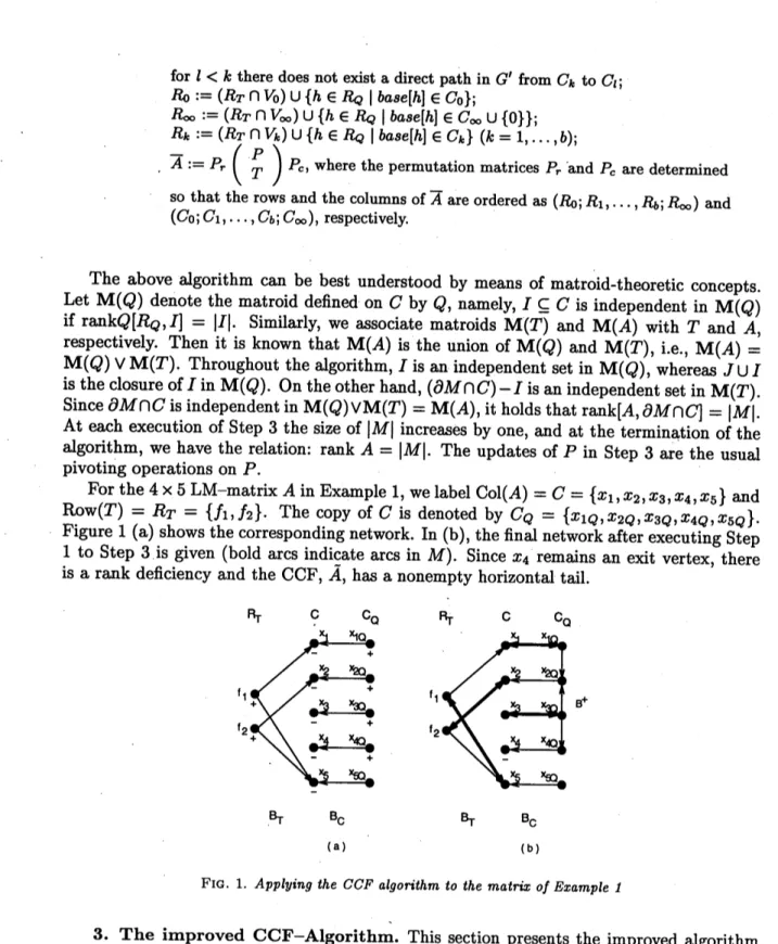
For the$4\cross 5$LM-matrix$A$in Example 1, welabelCo1_{$(A)=C=\{x_{1,2,3}XX,X_{4},x_{5}\}$}

and Row$(\tau)=R\tau=\{fi, f_{2}\}$

.

The copy of$C$ is denoted by

$C_{Q}=\{x_{1Q}, x_{2}Q,x3Q, x4Q, x_{5Q}\}$

.

Figure 1 (a) _{shows the corresponding network. In} _(b),_the_final_network_{after executing Step}

1 to Step 3 is given (bold

arcs

indicate

arcs

in $M$). Since $x_{4}$ remains an exit vertex, there

is arank deficiency and the CCF, $\tilde{A}$, has

a

nonempty horizontal tail.

$\mathrm{B}_{\mathrm{T}}$ $\mathrm{B}_{\mathrm{C}}$

$\mathrm{B}_{7}$ $\mathrm{B}_{\mathrm{C}}$

(a) (b)

FIG. 1. Applying the $CCFal_{\mathit{9}^{O\dot{n}\iota}}hm$ to the matfix ofExample 1

3. The improved CCF-Algorithm. This section presents the improved algorithm for computing the CCF. The $\mathrm{b}\mathrm{a}s$ic algorithm is

retained, but apractically faster algorithm is employed in order to improve solving theindependent assignment subproblem.

We will present _{this algorithm in two improving steps. In} _Section_3.1, _a_{revised version}

of the $\mathrm{b}\mathrm{a}s$

ic algorithm is introduced which incorporates two precalculation phases _called

Step A and Step $\mathrm{B}$, where Step A computes an

assignment in _{the subgraph induced} _by

$B_{T}$ and where Step $\mathrm{B}$ works on

$B_{C}$

.

Fora second improvement Step $\mathrm{B}$ is refined so that it

runs with higher efficiency (see Section3.2).

3.1. A revised CCF-algorithm. Recall that the $\mathrm{b}\mathrm{a}s$ic components

for computing

an independent assignment

are

path searching and matching update. _{Due to extensive}

updating processes the latter tends to be timecritical especially, as up until nowit has been

(4)

$\mathrm{f}\mathrm{a}s$ter algorithm lies in carrying out the update processes

more

carefully than the original

algorithm does. This is reasonable, since therearethreetypesof augmenting paths, namely

(1) those whichonly contain

arcs

$e\in B_{T}$,

(2) those with

arcs

$e\in B_{T}\cup B_{Q}$ (which initiate pivoting),

(3) those with

arcs

$e\in B_{T}\cup B_{Q}\cup B^{+}$ (which initiate pivoting and exchanges in the

base set and in $B^{+}$).

The strategy is to separate augmentings for the generic matrix $T$ (paths of the form (1))

from those

ones

for the elimination (pivoting) operations on $Q$ (paths of the form (2) and

(3)$)$ and to apply sophisticated routines in the respective augmenting processes. For the

algorithm it is also appropriate to start with a large assignment instead of the empty one.

Then certain augmenting steps

can

be unemployed until the final phase of the algorithm

where an optimal assignment has to be reached. We

can

apply this technique, since the structure of the underlying network makes it easy tocompute alarge initial assignment.

To be more concrete, the algorithm proposed here consists of the two preprocedures, Step A and Step $\mathrm{B}$, followed by the procedures of the original algorithm. In Step

$\mathrm{A}$, a

maximal (not necessarily maximum) matching $M_{B_{T}}$ in the subgraph induced on the vertex

set $R_{T}\cup C$ is computed using a simplegreedy strategy. Each

arc

$e\in M_{B_{T}}$ gives ashortest

path of length

one

whose augmenting will involve no pivoting. Step A adds the reversal of the

arcs

$e\in M_{B_{T}}$ to the assignment $M$ and updates the sets $S^{+}$ and $S^{-}$

.

The task of

Step $\mathrm{B}$ is to compute an initial set $I$ of independent columns whose size is possibly large.

For$I$, it chooses

a

maximal (not necessarily maximum) set of diagonal

arcs

$B_{C}’\subseteq B_{C}$ such

that each arc $(j_{Q},j)\in B_{C}$ connects an entrance with an exit vertex and such that the

set of corresponding matrix columns enjoys linear independency. In the revised algorithm, procedure Step $\mathrm{B}$ traverses the set $B_{C}$ of diagonal arcs

one

by one. Exactly those arcs

$(j_{Q},j)\in B_{C}$ with$j_{Q}\in S^{+}$ and$j\in S^{-}$ at the time of the traversalareselected for inclusion

in$I$

.

Before visiting the next arc, the corresponding pivotings are executed, sothat the list

ofdependent columns as wellas the set of entrance vertices can be updated accordingly. It is important to note that

arcs

of $B^{+}$, expressing exchangeability among columns of $I$ and $J$, are not needed in Step A and Step $\mathrm{B}$ and that their computation is therefore

omitted in either procedure. In the following step, however, $B^{+}$ will be computed for the

first time, since exchanges in the base set may become unavoidable for augmenting the

current assignment to optimality. Subsequently, the entire network will be submitted to the standard processes of path searching and matchingupdate (Step 2 and Step 3) of the original algorithm, before the ${\rm Min}-\mathrm{C}\mathrm{u}\mathrm{t}$-decomposition into strongly connected components

is called.

$\mathrm{R}_{-}$ $\Gamma^{\backslash }$. $\mathrm{r}_{-}$

$\mathrm{B}_{\mathrm{T}}$ $\mathrm{B}_{\mathrm{C}}$ $\mathrm{B}_{\mathrm{T}}$ $\mathrm{B}_{\mathrm{C}}$

$\langle$$\mathrm{a})$ (b)

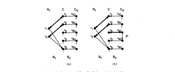
FIG. 2. Step $A$ and Step $B$ ofthe revised $al_{\mathit{9}^{O\dot{n}}}thm$

Example 3. We illustrate the revised algorithm on the matrix given in Example 1. In Figure 2 (a), we

see

the matching computed by Step A of the algorithm (bold lines). The

(5)

assignment after executing Step $\mathrm{B}$ which

covers arcs

of_{$B_{C}$} is displayed in (b). There, the

only arc contained in $B^{+}$ is shown

as

well. The initial assignment computed by Step A

and Step $\mathrm{B}$ is not optimal yet. The network will be submitted to the original algorithm

which augments the assignment along thepath$x_{1Q}arrow x_{1}arrow fiarrow x_{5}$, whichyields thefinal

optimal assignment as depicted in Figure 1 (b).

The revised algorithm for computing theCCF maynow be stated asfollows:

[Revised algorithm for the CCF ofa layered mixed matrix $\mathrm{A}$]

Step 1: $M:=\emptyset;I:=0;$ base$1^{i}$] $:=0(i\in R_{Q});P[i,j]:=Q_{j}|(i\in R_{Q}, j\in C)$

$S:=\mathrm{u}\mathrm{n}\mathrm{i}\mathrm{t}$ matrix oforder

$m_{Q}$;

$J:=$

{

$j\in C|P[i,j]=0$ for all $i\in R_{Q}$

}.

Step $\mathrm{A}:$ Let$\overline{M}$

bethe setofarcsofamaximal matching in the subgraph induced bythe vertex set $R\tau\cup C$;

$M:=\{(j, i)|(i,j)\in\overline{M}\}$;

$S^{-}:=C-\partial M;S_{T}^{+}:=R\tau-\partial M;S_{Q}^{+}:=\{j_{Q}\in C_{Q}|j\in C-J\};S^{+}:=S_{T}^{+}\cup S_{Q}^{+}$. Step $\mathrm{B}$: For all _{$(j_{Q},j)\in B_{C}$} do the$\mathrm{f}\mathrm{o}\mathrm{U}\mathrm{o}\mathrm{W}\mathrm{i}\mathrm{n}\mathrm{g}$:

{If

$j_{Q}\in S_{Q}^{+}$ and$j\in S^{-}$ do thefollowing:

{

$M:=M\cup(j,j_{Q});S_{Q}^{+}:=S_{Q}^{+}-\{j_{Q}\};S^{-}:=S^{-}-\{j\};I:=I\cup\{j\}$;

Find $h$ such that $base[h]=0$ and $P[h,j]\neq 0$; $base[h]:=j;w:=1/P[h,j]$;

$P[k, l]:=P[k, l]-w\cross P[k,j]\cross P[h, l](h\neq k\in R_{Q}, l\in C)$_; $S[k, l]:=S[k, l]-w\cross P[k,j]\cross S[h, l](h\neq k\in R_{Q}, l\in R_{Q})$ $J:=\{j\in C-I|\forall i:base[i]=0\Rightarrow P[i,j]=0\}$

$S_{Q}^{+}:=\{j_{Q}\in C_{Q}|j\in C-(I\cup J)\}\}\}$;

$S^{+}:=S_{T}^{+}\cup s_{Q}^{+};$

$B^{+}:=\{(i_{Q},j_{Q})|h\in R_{Q}, j\in J, P[h,j]\neq 0, i=base[h]\}$.

Step $\mathit{2}’$: Go to Step 3 of the original algorithm.

Improvements through the revised algorithm are based on the following facts: Firstly,

all shortest paths which have a length of 1 are detected in a single run. As for the original algorithm, these paths are detected in almost the same way, but Step A and Step $\mathrm{B}$ are

more straightforward, since they visit all arcs of $B_{T}$ (resp. $B_{C}$) only once. Secondly, as

already mentioned, a considerable amount of computation time is saved by postponing the computation and update of$B^{+}$ to the final augmenting phases, rather than repeatedly

computing$B^{+}$ already at the beginning. Thirdly,theseparationof augmentings for$B_{T}$from

those for $B_{C}$ makes it easier for each case, to decide

whi.ch

update steps become necessary

during the respectiveaugmentings.

3.2. Irnproving Step B. While it is easy to compute an initial assignment in $B_{T}$

in Step $\mathrm{A}$, Step $\mathrm{B}$ is a rather slow procedure. For each augmenting in _{$B_{C}$}, the

corre-sponding row elimination operations have to be carried out and accordingly the new

de-$\mathrm{p}\mathrm{e}\mathrm{n}\mathrm{d}\mathrm{e}\mathrm{n}\mathrm{C}\mathrm{e}/\mathrm{i}\mathrm{n}\mathrm{d}\mathrm{e}\mathrm{p}\mathrm{e}\mathrm{n}\mathrm{d}\mathrm{e}\mathrm{n}\mathrm{C}\mathrm{e}$structure has to be identified, i.e., $J$ has to be computed. As a

consequence the amount of computation as well as the computation time for $J$ increases

drastically with the matrix size.

One possible strategy for speeding up Step $\mathrm{B}$ is in a combinatorial relaxation for

com-puting an initial set $I$

.

That approach ignores the concrete values ofthe matrix entries in

favour of the combinatorial structure when it chooses an initial set of (yet not matched)

diagonal

arcs

for the set $I$

.

This procedure can work without $J$

.

(6)

the initial matching computed by Step A on the network $G$ of the independent assignment

subproblem. We define $R_{Q}=\mathrm{R}\mathrm{o}\mathrm{w}(Q)$ and, as usual, $C=\mathrm{C}\mathrm{o}1(A)$, and consider a directed

graph $G_{Q}=(V_{Q}, B_{Q})$ with the vertex set $V_{Q}=(C-\partial M)\cup R_{Q}$ and the

arc

set $B_{Q}=$ $\{(i,j)|i\in R_{Q},j\in C-\partial M, Q_{ij}\neq 0\}$

.

We then computea maximum matching$\overline{M}$in

$G_{Q}$

.

The set of columns of$Q$ (verticesin $C-\partial M$) covered by$\overline{M}$is agood candidate for the base

set $I$, though there remains the possibility of accidental numerical cancellation that

causes

linear dependency in $I$

.

In the latter case, the dependent columns willbe excluded from $I$

.

To beconcrete, each

arc

$(i,j)$ included in$\overline{M}$, where

$i\in R_{Q}$ and$j\in C-\partial M$, is used

as

a pivoting position, if the value of the entry is distinct from zero at the time ofpivoting (if

the entryequalszero, the column is not independent). Hence the$\mathrm{b}\mathrm{a}s\mathrm{e}$set $I$is composedof

allthe columns$j\in C$ whichare covered by the matching and whose corresponding pivoting element does not vanish during previous row eliminations. We will refer to this algorithm, which uses a combinatorial relaxation technique,

as

the relaxation algorithm. For nota-tional convenience, we do not distinguish vertices in $V_{Q}-R_{Q}$ and columns of$Q$

.

[Step $\mathrm{B}$ for the relaxation algorithm]

Step $\mathrm{B}:$ Let$\overline{M}$ beamaximum bipartite matching

on $G_{Q;}$

For all$j\in V_{Q}-R_{Q}$ do the $\mathrm{f}\mathrm{o}\mathrm{U}\mathrm{o}\mathrm{w}\mathrm{i}\mathrm{n}\mathrm{g}$:

{If

$j\in\partial\overline{M}$, find$i$ suchthat $(i,j)\in\overline{M}$;

If$P[i,j]\neq 0$, then do thefollowing:

{

$baSe[i]:=j;I:=I\cup\{i\};w:=1/P[i,j]$;

$P[k, l]:=P[k, l]-w\cross P[k,j1\cross P[i, l](i\neq k\in R_{Q}, l\in C)_{1}$ $S[k, l]:=S[k, l]-w\cross P[k,j1\cross S[i, l](i\neq k\in R_{Q}, l\in R_{Q})$ $\}\}$; $J:=$

{

$j\in C-I|$ Vi : $base[i]=0\Rightarrow P[i,j]=0$};

$S_{Q}^{+}:=\{j_{Q}\in CQ|j\in C-(I\cup j)\}$;

$S^{+}:=^{s^{+}}\tau\cup S_{Q}+$;

$B^{+}:=\{(i_{Q},j_{Q})|h\in R_{Q}, j\in J, P[h,j]\neq 0, i=base[h]\}$.

Wewillfinally introduceathird version of Step$\mathrm{B}$, which is simple

and fast, and installed for

our

newalgorithm. It gains its good performanceby the fact that we

can

dispense with the graph $G_{Q}$ aswellas thebipartite matching algorithm. This algorithm works

as

follows,

with

row

eliminations on the matrix $Q$

.

For each row $i$ of _$Q$ (after elimination), the first

entry $Q_{ij}$ with $Q_{ij}\neq 0$ is chosen for pivoting, where $j$ is not matched already. The base is

then enlarged bycolumn$j$ and the roweliminations

are

carried out, using_{$Q_{ij}$} as the

pivot-ing element. This quickly givesan initial assignment in $B_{C}$, whichis,

as

the $\mathrm{C}\mathrm{o}\mathrm{m}_{\mathrm{P}^{\mathrm{u}\mathrm{t}}\mathrm{a}1}\mathrm{a}\mathrm{t}\mathrm{i}\mathrm{o}\mathrm{n}$

experiments given in the next section will show, already close toan optimal

one.

[Step.B

for the new algorithm]

Step $\mathrm{B}$: For

$\mathrm{a}\mathrm{U}i\in R_{Q}$ dothefollowing:

{Find

$j\in C$such$j\not\in\partial M$ and $P[i,j1\neq 0$;

If such$j$ exists, do the following:

{

$base[i]:=j;I:=I\cup\{i\};w:=1/P[i,j]$;

$P[k, l]:=P[k, l]-w\cross P[k,j]\cross P[i, l](i\neq k\in R_{Q}, l\in C)$_;

$S1k,$ $l1:=S[k, l]-w\cross P[k,j1\cross s1^{i,l]}(i\neq k\in R_{Q}, l\in R_{\mathrm{Q}})\}\}$_;

$J:=$

{

$j\in C-I|\forall i:$ base$1i]=0\Rightarrow P[i,j]=0$}; $S_{Q}^{+}:=\{jQ\in C_{Q}|j\in C-(I\cup J)\}$;

$S^{+}:=s^{+}T\cup S_{Q}+$;

$B^{+}:=\{(iQ,jQ)|h\in R_{Q}, j\in J, P[h,j]\neq 0, i=base[h]\}$

.

This_{version has also the advantage that the pivoting elements}

_can

_{be determined quickly,} since for each rowthe first suitableentry is chosen for pivoting.

(7)

4. ComputationalExperiments. In the literature

we

couldfind only

a

fewexamples

where results on the combinatorial canonical fom have been reported. Murota [Mu87] considered matrices coming from chemical models and small matrices for the analysis of electronic networks. The latter includes

a

problem (Problem na18) with 6 resistors and 3

voltage controlled sources, where the coefficient matrix $A$ of the system ofequations _{to be}

solved was a layered mixed matrix of order 18. Emms [E94] also presented

some

results for the chemical model (reactor separator model EV-6). The system of$\mathrm{l}\mathrm{i}\mathrm{n}\mathrm{e}\mathrm{a}\Gamma/\mathrm{n}\mathrm{o}\mathrm{n}$-linear

equations to be solved involves 120 equations in 120 unknowns and also a singular matrix

(Problem p119) was formed out of EV-6 by deleting row 107 and column 109 from the corresponding mixed matrix. For our test series we additionally

ran

the algorithms

on

a

collection of matrices taken from the Harwell-Boeing databases (Problems IMPCOL and

$\mathrm{W}\mathrm{E}\mathrm{S}\mathrm{T})$[$\mathrm{D}\mathrm{G}\mathrm{L}89$, DGL92]. In these examples,

we regarded all integer coefficients whose modulus is less than or equal to 10

as

constant numbers and the others

as indeterminates.

Our computational experiments werecarriedout on a SUN

SPARCstation

10 $(125\mathrm{M}\mathrm{H}\mathrm{Z})$

using Mathematica, Version 2.2for

SPARC.

We used Mathematicaforits ability insymbolic computation and in order to provide an _{elegant code which is easy to follow for interested}

readers. Note, however,that the overhead incomputation timeis quite

enormous.

Moreover,

computation time is slightlyinfluenced _{by Mathematica’s internal data handling, where for}

instance the time neededfor operatingonthe network ($\mathrm{s}\mathrm{u}\acute{\mathrm{c}}\mathrm{h}$ as traversing)

is relatively high

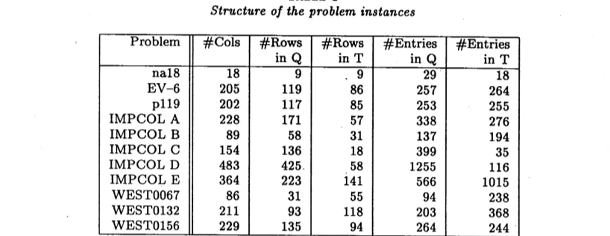
compared _{to the time needed for pivoting.} TABLE 1

$st_{\Gamma u}\mathrm{C}ture$ofthe problem instances

Table 1 summarizes properties of the input _{matrices. The size of the matrices} _ranges

from 18 to 483 and the number of

nonzero

coefficients from 47 to 1581. Table 2 describes the CCF _{for those matrices. From left to right it displays the rank of each matrix instance,}

the size of the horizontal and vertical tail, the total number of nonsingular square blocks, the number of those blocks of size

one

_{and finally the size of the largest square block.}

In

our

tests, we ran the original, the revised, the relaxation and the

new

algorithm

on

the abovetest matrices. Inorder to $\mathrm{e}\mathrm{v}\mathrm{a}\mathrm{l}\mathrm{u}\mathrm{a}\mathrm{t}^{\backslash }\mathrm{e}$thebehavior of the algorithms,we

investigated

three criteria: the number of pivoting operations, the number of base exchanges (both

Table 3) andthe computation time (Table 4).

Since the original and the revised algorithm augment the

as

signment along the

same

paths, _{the resulting numbers of pivotings and base exchanges} _are _identical. _On _{the other}

hand,onecanobserve that the improvedversions of Step$\mathrm{B}$ need less pivotingsasthey make

use

of the combinatorial structure of$Q$

.

Table 4 displays the computation time consumed by the algorithms. While already the revised algorithmconstantly outperformstheoriginalone, asignificant speedup is obtained under the$\mathrm{f}\mathrm{a}s$ter procedurefor Step$\mathrm{B}$, both in the relaxed and thenew

algorithm. Especially for large instances, one can observe a significant gain. We can also

see

that usually the

new

algorithm processes faster than the relaxation algorithm, except for IMPCOL $\mathrm{D}$ and

IMPCOL$\mathrm{E}$, where the number of rows in_$T$ is very

(8)

TABLE 2

$CCF$fortestmatrices

TABLE3

$N\mathrm{u}$mberofPivots and BaseExchanges

in $Q$

.

Theresults are confirmed in Table5which shows theeffect for the variants of Step $\mathrm{B}$

TABLE 4

Computation Time

in terms ofcomputation time.

From our experiments, we can conclude that there are two winners, namely the relaxed algorithm and the new algorithm, where in general, the new algorithm seems to behave better. Both versions provide a powerful algorithm for computing the CCF of a layered

mixed matrix and improve the original version significantly. We furtherexpect the running time to decrease considerably when implementing our code in a programming language

like $\mathrm{C}$ and using sophisticated pointer structures rather than exclusively working on

data structures $\mathrm{b}\mathrm{a}s$ed on Mathematica lists.

In order to further exploit what really happens when executing the algorithm

on

the above problems, we compiled some additional computational details. Table 6 describes,

(9)

TABLE 5

Computation Time_forStep $B$

how Step A and Step $\mathrm{B}$ (combinedwith the

new

algorithm) behave on the given problems.

The table lists the number of

arcs

of the assignment initially computed on columns of $Q$

($\# B_{C}$-Assignment) and rows of$T.$($\# B_{T}$-Assignment) and thefinal distribution of the

assignment on $Q$ and $T$

.

Column Augm. calls gives the number of augmentings along

shortest paths which are needed in order to yield the final independent assignment. We also calculated the change in the number of nonvanishing coefficients during the matrix transformation (Entries). The$1\mathrm{a}s\mathrm{t}$ three columns list thecomputationaltime consumed by

Step A and Step $\mathrm{B}$ and the time needed for the augmentingphase and the decomposition.

TABLE6

Applying the new algorithm

From

our

computational experiments we

can

draw the conclusion that the procedures

StepA and Step $\mathrm{B}$ producegood starting assignments such that the number of calls of Step 2

and Step3 (which are rathertime consumingprocedures) couldremain small. The findings of the test further indicate that the computation ofaninitialassignment is dominated by the elimination operations, so that thealgorithm still spends much ofthecomputation time for

Step B. Ontheotherhand, acomparableamountofcomputationtimeisconsumedinthefew augmentingsteps from the initial assignment to the optimal one. Also, the decomposition

phaseis still relativelyslow, since

we

did not put mucheffort in its implementationand the data structures.

A. Appendix: ImplementationManual. Theprogramcode ofourimplementation

for computing the CCF is available via anonymousftp from $\mathrm{w}\mathrm{w}\mathrm{w}$

.

kurims. kyoto-u.$\mathrm{a}\mathrm{c}$

.

jp.

Please change to the directory$\mathrm{p}\mathrm{u}\mathrm{b}/\mathrm{p}\mathrm{a}\mathrm{p}\mathrm{e}\mathrm{r}/\mathrm{m}\mathrm{e}\mathrm{m}\mathrm{b}\mathrm{e}\mathrm{r}/\mathrm{m}\mathrm{u}\mathrm{r}\mathrm{o}\mathrm{t}\mathrm{a}$ and read the READMEfile.

Alter-nativelyyoucancheck thehomepageunderhttp:$//\mathrm{w}\mathrm{w}\mathrm{w}$

.

kurims. kyoto-u.

$\mathrm{a}\mathrm{c}.\mathrm{j}\mathrm{p}/\sim \mathrm{m}\mathrm{u}\mathrm{r}\mathrm{o}\mathrm{t}\mathrm{a}$

.

Thegivendirectories include thenewalgorithm which–asamathematica package–is named$\mathrm{c}\mathrm{c}\mathrm{f}.\mathrm{m}$

.

Also,weprovideafileccfstat.$\mathrm{m}$which creates, inadditiontocomputing the

(10)

CCF, a file stat.$\log$ ofcomputation statistics. For demonstrating purposes, all matrices

used in the computational experiments aregiven in

a

subdirectory data.

When running

a

mathematica session, include the package ccf.m (or ccfstat.m) by simply typing $”<<\mathrm{c}\mathrm{c}\mathrm{f}.\mathrm{m}$” in the Mathematicaprompt. The variables used in the code

are

protected such that

we

do not worry about conflicting variable setting caused by previous computations. Typing “$\mathrm{C}\mathrm{C}\mathrm{F}\lceil filename$]” will execute the algorithm on the input matrix

given in

_filename.

The resulting decomposition will be displayedon the

screen

and in a file

$\mathrm{c}\mathrm{c}\mathrm{f}$

.

out in asparse matrix format.

The sparse matrixformat usedfor the input matricesas wellasfor the file $\mathrm{c}\mathrm{c}\mathrm{f}$

.

out is as

follows: The first line gives the number of columns. The second and the third line contain the number of

rows

in $Q\mathrm{a}\mathrm{n}\dot{\mathrm{d}}$in_$T$, respectively. Separated

by aline withazero, the matrix coefficients

are

described. Each line contains, from left to the right, the number of the row, the number of nonvanishing entries in that row and a pair $(j, m_{j})$ consisting of the column

number for each such entry

as

well

as

the value of that coefficient. For the submatrix $T$for

simplicity, the $\mathrm{s}\mathrm{y}\mathrm{m}\mathrm{b}_{\mathrm{o}\mathrm{I}}$entries all get the value

zero.

REFERENCES

[BR91] R. A. BRUALDI AND H. J. RYSER, $Combinaio\dot{-}al$ _Matrix _Theory, _{Cambridge University}_Press,

London, 1991.

[DER86] I. S. DUFF, A. M. ERISMAN AND J. K. REID, Discrete Methods_forSparse Matrices, Clarendon

Press, Oxford, 1986.

[DGL89] I. S. DUFF, R. G. GRIMES AND J. G. LBWIS, Sparse matrix test problems, ACM Trans. Math. Software, 15 (1989),pp. 1-14.

[DGL92] I. S. DUFF, R. G. GRIMES AND J. G. LEWIS, Users’ Guide _for the Harwell-Boeing Sparse

Matrix Collection(Release I), $\mathrm{T}\mathrm{R}/\mathrm{P}\mathrm{A}/92/86$, CERFACS, Toulouse Cedex, France, 1992.

[DR78] I. S. DUFFAND J. K. REID, An implementation _of$\tau_{a\dot{\eta}a}n^{r}S$ algorithmfor the block

triangular-ization _ofa matrix,ACM Trans. Math. Software,4 (1978),pp. 137-147.

[DM59] A. L. DULMAGEANDN. S.MENDELSOHN, Astructure theory_ofbipartite graphs_offinite exterior

dimension,Trans. Roy.Soc. Canada, SectionIII, 53(1959), pp. 1-13.

[E94] N. R. E. EMMS, AnImplementation _ofthe Combinatorial Canonical FomDecomposition

Al-gonthm_forLayered Mixed Matfices, Dissertation forMaster Thesis, Kyoto Univ., 1994.

[EGLPS87] A. M. ERISMAN, R. G. GRIMES, J. G. LEWIS, W. G. POOLE, JR. AND H. D. SIMON,

Evalu-ation _oforderings_forunsymmetric sparse matrices, SIAM J. Sci. Stat. Comput., 8 (1987),

pp. 600-624.

[Gu76] F. GUSTAVSON, Findingthe Block Lower TriangularForm_ofa Sparse Matrix,inSparseMatrix

Computations,J. R. Bunch andD. J. Rose, eds., AcademicPress, 1976,pp. 275-289.

[Ho76] T. D. HOWELL, Partitioning using PAQ, in Sparse Matrix Computations, J. R. Bunch and

D. J. Rose, eds.,AcademicPress, 1976, pp.23-37.

[Mu87] K. MUROTA, Systems Analysis by Graphs and Matroids –Stfuctural Solvability and

Controlla-bility, Springer-Verlag, 1987.

[Mu93] K. MUROTA, Mixed Matrices –Irreducibility and Decomposition, in Combinatorial and Graph

Theoretic Problems in Linear Algebra, R. A. Brualdi, S. Friedland and V. Klee, eds., The IMA Volumes in Mathematics and Its Applications, Vol.50,_{Springer-Verlag 1993, pp. 39-71.} [Mu96] K. MUROTA,Structuralapproachinsystems analysis bymixed$mat\dot{\cap}ces-An$_exposition_for_index

ofDAE,in ICIAM 95(Proc. ThirdIntern. Congr. Indust.Appl. Math.,Hamburg, Germany,

July 3-7, 1995), K. Kirchg\"assner, O. Mahrenholtz and R. Mennicken, eds., Mathematical

Research, Vol. 87, AkademieVerlag, 1996, pp. 257-279.

[MI85] K. MUROTAANDM. IRI, Structuralsolvability _ofsystems _ofequations–A mathematical

formu-lation_for distinguishing accurate andinaccurate numbers in structural analysis _ofsystems, JapanJ. Appl. Math., 2 (1985), pp. 247-271.

[MIN87] K. MUROTA, M. IRIAND M. NAKAMURA, Combinatorialcanonical_{form of}layered mixed

matri-ces andits application to block-triangularization_ofsystems _ofequations, SIAMJ. Algebraic DiscreteMethods, 8(1987),pp. 123-149.

[PF90] A. POTHEN AND C. J. FAN, Computing the block triangular_{fom of} a sparse matrix, ACM Trans. Math. Software, 16 (1990),pp. 303-324.

[YTK81] K. YAJIMA, J. TSUNEKAWA AND S. KOBAYASHI, On equation-based dynamic simulation, Proc. WorldCongr. Chem. Eng., Montreal, V (1981).