A Simple Design of Chaotic Binary Sequences with Prescribed Auto-Correlation Properties Based on Piecewise Linear Onto Maps (5th Workshop on Stochastic Numerics)

(1)

ASimple Design

of

Chaotic Binary

Sequences

with

Prescribed

_{Auto-Correlation}

_Properties

Based

on

Piecewise

Linear

Onto Maps

Akio

TSUNEDA

Department ofElectrical and Computer Engineering,

Kumamoto University, Japan

2-39-1 Kurokami, _{Kumamoto 860-8555,} _Japan

Tel: +81-96-342-3853, Fax: +81-96-342-3630

E-mail : t suneda@eecs._{kumamoto-u.ac.jp}

Abstract: This paper describes simple _{design methods of chaotic binary sequences with}

prescribed _{aut0-correlation properties} _{including higher-0rder statistics. We employ}

one-dimensionalpiecewiselinearontomaps and simplethreshold functionsforgenerating such

sequences. Some examples of such designs are also _{given. Furthermore, bounds on such}

statistics are discussed and compared to the result for general binary random variables.

1Introduction

Simpledeterministicsystems_{can exhibit very complex and random}_behavior_called _chaos.

Such phenomena are very interestingin both oftheoretical and engineeringpoint of view.

One of the most _{useful applications of chaos is arandom number} _generator _{which is}

re-quired in several engineering applications such as Monte Carlo simulations, spread

spec-trum communications, and cryptosystems. In many kinds of pseudorandom numbers,

binary sequences are most useful in such digital communicationsystems. The best known

class of binary sequences is the s0-called linear feedback shift register (LFSR) sequences

such as $\mathrm{M}$-sequences, Gold sequences, and

Kasami sequences [1].

As quite different methods from LFSR_{sequences, there have been several attempts to}

use chaotic sequences which are generated by one-dimensional nonlinear maps. Though

achaotic sequence itself is real-valued, it can be easily transformed into binary sequences

by appropriate threshold functions. In applications _{of such chaotic sequences,} _theoretical

evaluation and design of statistical properties of such sequences are very important

be-causethere are many kinds ofchaotic sequences with various properties which depend on

their deterministicsystems.

Design ofmany chaotic sequences of $i.i.d$. (independent and identically _distributed)

binary random variables from asingle chaotic real-valued sequence generated by aclass of

one-dimensional maps has been established [2]. _{Ageneralized version of such design has}

also been given [3]. _{Sequences of i.i.d. binary random variables are very useful as random}

numbers. However _{non-i.i.d. sequences, which have} _some _{correlations dependent on the}

chaotic maps and quantizationfunctions, are also useful in someapplications. Actually, it

has been shown that sequences with exponentially vanishingaut0-correlations have better

performance in asynchronous $\mathrm{D}\mathrm{S}/\mathrm{C}\mathrm{D}\mathrm{M}\mathrm{A}$ systems than i.i.d. sequences $[4],[5]$. Thus, it is

very important to design chaotic sequences _{with prescribed statistical properties}

数理解析研究所講究録 1240 巻 2001 年 192-203

(2)

Design of chaotic real-valued orbits with prescribed statistical properties have b$\mathrm{e}\mathrm{e}\mathrm{n}$

discussed in [6]. Also, design of dynamical systems which generates an arbitrarily

pre-scribed tree sourceby using piecewiselinear maps has beengiven [7]. We also remarkthat

Kalman already gave aprocedure for embedding aMarkov chain into chaotic dynamics

of piecewise linear maps $[8],[9]$.

In this paper, we present simple design methods to obtain chaotic binary sequences

with prescribed aut0-correlation properties, including higher-0rder statistics, based on

piecewise linear onto maps with auniform invariant measure [10]-[12]. We also use a

simple threshold function for generating chaotic binary sequences from

areal-valued

one.

2One-Dimensional

Maps

and

Chaotic

Binary

Sequences

One-dimensional

nonlinear difference equation

$x_{n+1}=\tau(x_{n})$, $x_{n}\in I=[d, e]$, $n=0,1,2$,$\cdots$ , (1)

can produce achaotic sequence $\{x_{n}\}_{n=0}^{\infty}$, where $x_{n}=\tau^{n}(x_{0})$. The ensemble-average

defined by

$\langle G\rangle=\int_{I}G(x)f^{*}(x)dx$ (2)

is very useful in evaluating statistics of $\{G(\tau^{n}(x))\}_{n=0}^{\infty}$ under the assumption that $\tau(\cdot)$

is mixing on I with respect to an absolutely continuous invariant measure, denoted by

$\mathrm{g}\mathrm{i}(\mathrm{x})dx$. In this paper, we employ piecewise monotonic onto maps with

$N_{\tau}$ subintervals.

We now define the Perron-Frobenius (PF) operator $P_{\tau}$ of the map $\tau$ with an interval

$I=[d, e]$ by

$P_{\tau}G(x)= \frac{d}{dx}\int_{\tau^{-1}([d,x])}G(y)dy$ (3)

which can be rewritten as

$P_{\tau}G(x)= \sum_{i=1}^{N_{\mathcal{T}}}|g_{i}’(x)|G(g_{i}(x))$ (4)

for piecewise monotonic onto maps, where $g_{i}(x)$ is the $i$-th preimage ofthe map $\tau(\cdot)[13]$.

This operator is very useful in evaluating the correlation functions because it has the

following important property:

$\int_{I}G(x)P_{\tau}\{H(x)\}dx=\int_{I}G(\tau(x))H(x)dx$. (5)

Areal-valued chaotic sequence generated by such amap is easily

transformed

into a

binary sequence by athreshold function defined by

$\Theta_{t}(x)=\{$ 0 $(x<t)$ (6)

1 $(x\geq t)$.

We will discuss statistical properties of abinary sequence $\{\Theta_{t}(\tau^{n}(x))\}_{n=0}^{\infty}$ generated by

the threshold function

(3)

3 _{Chaotic Binary}

_Sequences

_with

_Prescribed

AutO-Correlation

Properties

3.1

$2\mathrm{n}\mathrm{d}$

-Order

AutO-Correlation

Firstly, we define the $2\mathrm{n}\mathrm{d}$-order

aut0-correlation function ofasequence $\{G(\tau^{n}(x))\}_{n=0}^{\infty}$ by

$\rho(\ell;G)=\int_{I}(G(x)-\langle G\rangle)(G(\tau^{\ell}(x))-\langle G\rangle)f^{*}(x)dx$. ₍₇₎

For an i.i.d. binary sequence $\{B(\tau^{n}(x))\}_{n=0}^{\infty}$ as given in [2], we have

$\rho(\ell;B)=(\langle B\rangle-\langle B\rangle^{2})\delta(\ell)$, (8)

where $8(0)=1$ and $\delta(\ell)=0$ for $\ell>1$.

Now, we consider piecewise linear (PL) onto _{maps whose mapping} _function $\tau_{i}(\cdot)$ in

each subinterval $I_{i}(i=1,2, \cdots, N_{\tau})$ is given by

$\tau_{i}(x)=a_{i}x+b_{i}$, $|a_{i}|>1$, $\tau_{i}$ : $I_{i}arrow I$ (onto). (9)

Without any loss of generality, we

assume

$I=[0,1]$

.

_{For such maps, the} _{invariant density}

function $f^{*}(x)$ is constant such that _{$\int_{I}f^{*}(x)dx=1$}, that is, _$f^{*}(x)=1$_{. We}

call eq.(9) the

onto _{condition through this paper. Thus, we} _{can obtain} _the _{following lemma.}

Lemma 1: For the piecewise linear onto maps given by (9), we can get

$P_{\tau} \{(\Theta_{t}(x)-\langle\Theta_{t}\rangle)f^{*}(x)\}=\frac{1}{a_{r}}(\Theta_{\tau(t)}(x)-\langle\Theta_{\tau(t)}\rangle)f^{*}(x)$ (10)

where $t\in I_{r}$.

By using _{the above lemma, we can obtain the} _{following theorem.}

Theorem 1: Let $c$ be afixed point of the map satisfying

$\tau(c)=c$. If we employ the

threshold $c(\in I_{r})$, we have

$\rho(\ell;\Theta_{c})=\frac{\rho(0,\Theta_{c})}{a_{r}^{\ell}}.=\frac{\langle\Theta_{c}\rangle-\langle\Theta_{c}\rangle^{2}}{a_{r}^{\ell}}$. (11)

It should be noted that eq.(ll) _{is independent of the} _{mapping functions} $\tau_{i}(\cdot)(i\neq r)$.

Thus, we can control the aut0-correlation property _{of the chaotic binary sequence by} $c$

and $a_{r}$, where we can use arbitrary values of

$a_{r}$ whose absolute value is greater than 1.

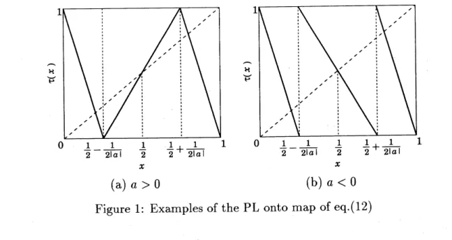
Example 1: Define apiecewise linear onto map with $I=[0,1]$ by

$\tau(x)=\{$

$\frac{2|a|}{ax-1-|a}1\frac{a-11^{x+}}{2}$

$(0 \leq x<\frac{1}{2}-\frac{1}{2|a|})$

$( \frac{1}{2}-\frac{1}{2|a|}\leq x<\frac{1}{2}+\frac{1}{2|a|})$

$\frac{2|a|}{1-|a|}(x-1)$ $( \frac{1}{2}+\frac{1}{2|a|}\leq x\leq 1)$

$|a|>1$

.

₍₁₂₎

Examples of the above map are shown in Fig.1. According to Theorem 2, the

aut0-correlation function ofabinary sequence $\{\ominus\frac{1}{2}(\tau^{n}(x))\}_{n=0}^{\infty}$ obtained by the PL onto map

ofeq. (12) is given by

$\rho(\ell;\Theta_{\frac{1}{2}})=\frac{1}{4a^{\ell}}$.

(13)

(4)

$x$ $x$

(a) $a>0$ (b) $a<0$

Figure 1: Examples of the PL onto map of eq.(12)

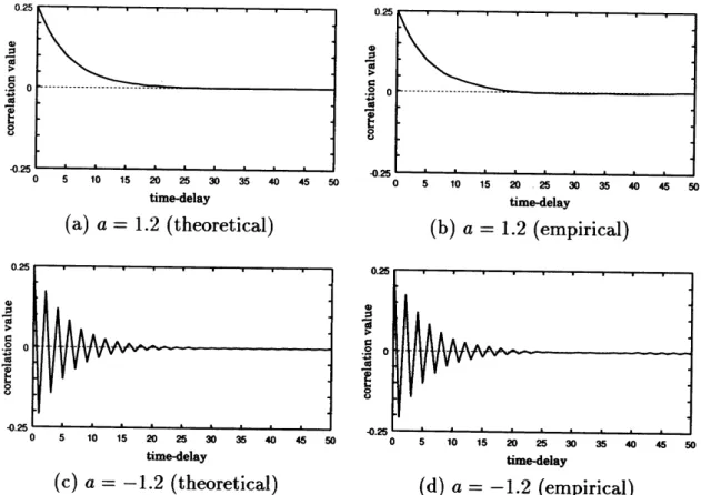
Figure 2shows examples oftheoretical and empirical correlation values of$\{\Theta_{\frac{1}{2}}(\tau^{n}(x))\}_{n=0}^{\infty}$

generatedby PLontomaps of eq.(12), where empiricalvalues are obtained by acomputer.

We can find that the theoretical and empirical values are in good agreement with each

other.

3.2 Run-Probability

When $B(\cdot)$ is abinary ({0,

1}-valued)function,

the probability of$m$ successive l’s in the

binary sequence $\{B(\tau^{n}(x))\}_{n=0}^{\infty}$ is given by

$P_{m}(B)= \int_{I}B(x)B(\tau(x))\cdots B(\tau^{m-1}(x))f^{*}(x)dx$, (14)

which is one of higher-0rder statistics and is also useful for some statistical tests [14].

We call this probability run-probability. Of course, if the sequence is i.i.d., we have

$P_{m}(B)=\langle B\rangle^{m}$.

Here, again, considerthepiecewise linear onto maps givenby (9). We give the following

theorem.

Theorem 3: Let $t$ be avalue such that $t<\tau(t)$,$t<\tau^{2}(t)$,$\cdots$,$t<\tau^{p-1}(t)$ and $t\geq\tau^{p}(t)$.

Then, for the piecewise linear onto maps given by (9), we have

$P_{m}( \Theta_{t})=(\prod_{i=0}^{p-1}\frac{1}{a^{(i)}})P_{m-p}(\Theta_{t})+\sum_{j=1}^{p}(\prod_{i=0}^{j-2}\frac{1}{a^{(i)}})(\langle\Theta_{\tau^{f1}(t)}-\rangle-\frac{\langle\Theta_{\tau^{j}(t)}\rangle}{a^{(j-1)}})P_{m-j}(\Theta_{t})$ (15)

where $a^{(i)}$ is the slope of the mapping function of the subinterval in which $\tau^{i}(t)$ exists.

Proof: Using eq.(10), we can write

$P_{m}( \Theta_{t})=\int_{I}P_{t}(x)f^{*}(x)\}\Theta_{t}(x)\cdot\Theta_{t}(\tau^{m-2}(x))dx=\int_{I}\{\frac{\tau\{\Theta 1}{a^{(0)}}(\Theta_{\tau(t)}(x)-\langle\Theta_{\tau(t)}\rangle)f^{*}(x)\}\Theta_{t}(x)\cdots\Theta_{t}(\tau^{m-2}(x))dx$

(5)

timedelay

(a) $a=1.2$ _{(theoretical)} _(b) _$a=1.2$ _(empirical)

(c) $a=-1.2$ (theoretical) _{(d) $a=-1.2$} _(empirical)

Figure 2: ontocorrelation functions of$\{\Theta_{\frac{1}{2}}(\tau^{n}(x))\}_{n=0}^{\infty}$ generated by PL onto maps with

$a=\pm 1.2$.

$= \frac{1}{a^{(0)}}\int_{I}\Theta_{\tau(t)}(x)\Theta_{t}(\tau(x))\cdots\Theta_{t}(\tau^{m-2}(x))f^{*}(x)dx$

$+( \langle\ominus_{t}\rangle-\frac{\langle\Theta_{\tau(t)}\rangle}{a^{(0)}})P_{m-1}(\Theta_{t})$ (16)

and thus by induction we have eq.(15).

Remark: For maps with the EDP, $P_{m}(\ominus_{t})$ as in Theorem 3is obtained by substituting

$a^{(i)}=s((\tau^{i})’(t))N_{\tau}$ into eq.(15).

From Theorem 3, we find that the run-probability of Is in the sequence is also

control-lableto some extent. Note that eq.(15) _{is independent of slopes of the mapping}_functions

of the subintervals in which $\tau(:t)$ does not exist. We give simple design examples based

on piecewise linear onto maps as follows.

Example 2: For $t\geq\tau(t)$ and $t\in I_{r}$, we have

$P_{m}( \Theta_{t})=(\frac{1-\langle\ominus_{\tau(t)}\rangle}{a_{r}}+\langle\Theta_{t}\rangle)P_{m-1}(\Theta_{t})$ (17)

$=( \frac{1-\langle\Theta_{\tau(t)}\rangle}{a_{r}}+\langle\Theta_{t}\rangle)^{m-1}\cdot\langle\Theta_{t}\rangle$

(18)

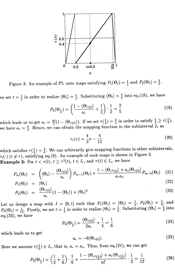
Let us design amap with $I=[0,1]$ _{such that Pi}_{Qt) $= \langle\ominus_{t}\rangle=\frac{1}{2}$ and P2(&t) $= \frac{2}{5}$. Firstly

(6)

$x$

Figure 3: An example of PL onto maps satisfying $P_{1}( \Theta_{t})=\frac{1}{2}$ and $P_{2}( \Theta t)=\frac{2}{5}$.

we set $t= \frac{1}{2}$ in order to realize $\langle\Theta_{t}\rangle=\frac{1}{2}$

.

Substituting $\langle\Theta_{t}\rangle=\frac{1}{2}$ into eq.(18), we have

$P_{2}( \Theta_{\frac{1}{2}})=(\frac{1-\langle\Theta_{\tau(t)}\rangle}{a_{r}}+\frac{1}{2})\cdot\frac{1}{2}=\frac{2}{5}$ (19)

which leads us to get $a_{r}= \frac{10}{3}(1-\langle\Theta_{\tau(t)}\rangle)$. Ifwe set $\tau(\frac{1}{2})=\frac{2}{5}$ in order to satisfy $\frac{1}{2}\geq\tau(\frac{1}{2})$,

we have $a_{r}= \frac{4}{3}$

.

Hence, we can obtain the mapping function in the subinterval

$I_{r}$ as

$\tau_{r}(x)=\frac{4}{3}x-\frac{4}{15}$ (20)

’

Example 3: For $t<\tau(t)$, $t\geq\tau^{2}(t)$, $t\in I_{r}$, and $\mathrm{r}(\mathrm{t})\in I_{s}$, we have

$P_{m}( \Theta_{t})=(\langle\Theta_{t}\rangle-\frac{\langle\Theta_{\tau(t)}\rangle}{a_{r}})P_{m-1}(\Theta_{t})+\frac{1-\langle\Theta_{\tau^{2}(t)}\rangle+a_{s}\langle\Theta_{\tau(t)}\rangle}{a_{r}a_{s}}P_{m-2}(\Theta_{t})$ (21) $P_{1}( \Theta_{t})P_{2}(\Theta_{t})==\frac{\langle\Theta_{t}\rangle\langle\Theta_{\tau(t)}\rangle}{a_{r}}(1-\langle\Theta_{t}\rangle)+\langle\Theta_{t}\rangle^{2}$ (22) (23) $\mathrm{L}\mathrm{e}\mathrm{t}\mathrm{u}\mathrm{s}\mathrm{d}\mathrm{e}\mathrm{g}\mathrm{n}\mathrm{a}\mathrm{m}\mathrm{a}\mathrm{p}\mathrm{w}\mathrm{i}\mathrm{t}\mathrm{h}I=[0, 1]\mathrm{s}\mathrm{u}\mathrm{c}\mathrm{h}\mathrm{t}\mathrm{h}\mathrm{a}\mathrm{t}P_{1}(\Theta_{t})=\Theta_{t}\rangle=\frac{1}{2,\mathrm{t}},P_{2}(\Theta_{t})=\frac{1}{6},\mathrm{a}\mathrm{n}\mathrm{d}P_{3}(\Theta_{t})=\frac{\mathrm{s}_{1}\mathrm{i}}{12}.\mathrm{F}\mathrm{i}\mathrm{r}\mathrm{s}\mathrm{t}1\mathrm{y}\mathrm{w}\mathrm{e}\mathrm{s}\mathrm{e}\mathrm{t}t=\frac{1}{2}\mathrm{i}\mathrm{n}\mathrm{o}\mathrm{r}\mathrm{d}\mathrm{e}\mathrm{r}\mathrm{t}\mathrm{o}\mathrm{r}\mathrm{e}\mathrm{a}1\mathrm{i}\mathrm{z}\mathrm{e}\langle\Theta_{t}\rangle=\frac{1\langle}{2}$

.

$\mathrm{S}\mathrm{u}\mathrm{b}\mathrm{s}\mathrm{t}\mathrm{i}\mathrm{u}\mathrm{t}\mathrm{i}\mathrm{n}\mathrm{g}\langle\Theta_{t}\rangle--\frac{1}{2}\mathrm{i}\mathrm{n}\mathrm{t}\mathrm{o}$ eq. (23), we have $P_{2}( \Theta_{\frac{1}{2}})=\frac{\langle\Theta_{\tau(t)}\rangle}{2a_{r}}+\frac{1}{4}=\frac{1}{6}$ (24)

which leads us to get

$a_{r}=-6\langle\Theta_{\tau(t)}\rangle$

.

(25)

Here we assume $\tau(\frac{1}{2})\in I_{r}$, that is, $a_{r}--a\mathrm{s}.$ Thus, from eq.(21), we can get

$P_{3}( \Theta_{\frac{1}{2}})=(\frac{1}{2}+\frac{1}{6})\cdot\frac{1}{6}+\frac{1-\langle\Theta_{\tau^{2}(\frac{1}{2})}\rangle+a_{r}\langle\Theta_{\tau(\frac{1}{2})}\rangle}{a_{r}^{2}}\cdot\frac{1}{2}=\frac{1}{12}$. (26)

197

(7)

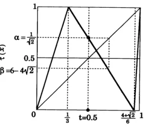
$x$

Figure 4: An example of PL onto maps satisfying $P_{1}( \Theta_{t})=\langle\Theta_{t}\rangle=\frac{1}{2}$, $P_{2}( \ominus_{t})=\frac{1}{6}$, and

$P_{3}( \Theta_{t})=\frac{1}{12}$.

Put $\alpha=\tau(\frac{1}{2})$ and $\beta=\tau^{2}(\frac{1}{2})$. Then we have

$\langle\ominus_{\tau(\frac{1}{2})}\rangle$ $=$ $1-\alpha$ (27) $\langle\Theta_{\tau^{2}(\frac{1}{2})}\rangle$ $=$ $1-\beta$ (28)

$\tau_{r}(x)$ $=a_{r}(x- \frac{1}{2})+\alpha$ ₍₂₉₎

$\tau_{\gamma}(\alpha)$ $=\beta$.

(30)

Using _{eq.(25)-(30), we can get each value of the} _parameters _and _obtain _the _mapping

function in the subinterval $I_{r}$ as

$\tau_{r}(x)=3(\sqrt{2}-2)x+3-\sqrt{2}$_. ₍₃₁₎

We can also arbitrarily give mapping functions in other subintervals, $\tau_{i}(\cdot)(i\neq r)$,

satis-fying eq.(9). An example of such maps is shown in Figure 4.

4Discussion

of

_{Run-Probability}

Now consider the simplest case $p=1$ in eq.(15), that is, the case ofeq.(18). Further, we

focus our attention on the case $m=2$

.

_Using $\langle\Theta_{t}\rangle=1-t$, we have

$P_{2}( \ominus_{t})=(\frac{\tau(t)}{a_{r}}+1-t)(1-t)$. (32)

We consider bounds on the run-probability $P_{2}(\Theta_{t})$ given by eq.(32). There are three

parameters$t$, $\tau(t)$,and$a_{r}$ which determine the value of$P_{2}(\Theta_{t})$

.

However, theseparameters

are not _{completely independent each other since the} _onto _condition _eq.(9) _and $t\geq \mathrm{r}(\mathrm{t})$

must be satisfied as long as eq.(32) is used. Hence, eq.(32) should have some bounds

which are of our main interest in this section. Thus, we theoretically investigate such

bounds for agiven $P_{1}(\ominus_{t})=\langle\ominus_{t}\rangle$ ($i.e.$, agiven $t$).

(8)

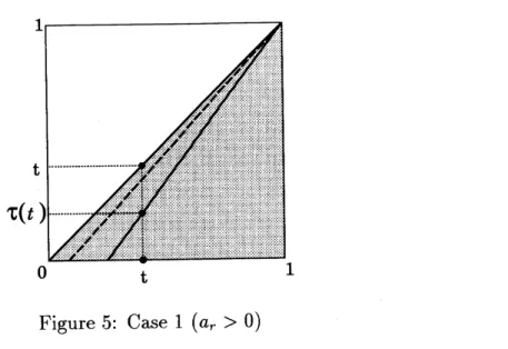
Figure 5: Case 1 $(a_{r}>0)$

To do this, we consider the following cases. Note that each case corresponds to each

of Figures 5-8. In these figures, the coordinate $(t, \mathrm{r}(\mathrm{t})$, which is one of parameters

determining the mappingfunction, must be located in shaded area in order to satisfy the

given conditions.

$\bullet$ Case 1: $a_{r}>0(\mathrm{F}\mathrm{i}\mathrm{g}.5)$

In this case, obviously, the minimum value of $P_{2}(\Theta)$ is $(1 -t)^{2}$ to be obtained for

$\mathrm{o}\mathrm{n}P_{2}(\Theta)\tau(t)=0$

,

condition. As shown in Fig.5, the mapping function $\tau_{r}(x)$ is alinear one with $\tau_{r}(t)=\tau(t)$

and Tr(t) $=1$, whose slope $a_{r}$ is given by

$a_{r}= \frac{1-\tau(t)}{1-t}$. (33)

Thus, the upper bound is $1-t$ to beobtained for $\tau(t)=t$. Note that when $\tau(t)=1$, that

is, $a_{\gamma}=1$, the map is no longer chaotic. Thus, in this case, we have

$P_{1}(\Theta_{t})^{2}\leq P_{2}(\Theta_{t})<P_{1}(\Theta_{t})$. (34)

$\bullet$ Case 2-1: $a_{r}<0$, $t \geq\frac{1}{2}$, and $\tau(t)>1-t(\mathrm{F}\mathrm{i}\mathrm{g}.6)$

In this case, the upper bound on $P_{2}(\Theta)$ is $(1-t)^{2}$ to be obtained for $a_{r}arrow\infty$. Next,

consider the most correlated case. As shown in Fig.6, the mapping function $\tau_{r}(x)$ is a

linear one with $\tau_{r}(t)=\tau(t)$ and $\tau_{r}(1)=0$ for the most correlated case where the absolute

value of the slope of $\tau_{r}(x)$, $|a_{r}|$, is closest to 1while keeping the onto condition. In this

case, we have

$a_{r}=- \frac{\tau(t)}{1-t}$. (35)

Substituting eq.(35) into eq.(32), we can get $P_{2}(\Theta_{t})=0$ which is independent of$\tau(t)$ and

is the minimum value in this case. Hence we have

$0\leq P_{2}(\Theta_{t})<P_{1}(\Theta_{t})^{2}$. (36)

$\bullet$ Case 2-2: $a<0$, $t \geq\frac{1}{2}$, and $\tau(t)\leq 1-t(\mathrm{F}\mathrm{i}\mathrm{g}.7)$

(9)

Figure 6: Case 2-1 ($a_{r}<0$, $t \geq\frac{1}{2}$, and _{$\mathrm{r}(\mathrm{t})>1-t$})

Figure 7: Case 2-2 ($a_{r}<0$, $t \geq\frac{1}{2}$, and $\tau(t)\leq 1-t$)

In this case, the maximumvalue of $P_{2}(\Theta)$ is also $(1-t)^{2}$ to be obtained for _{$\mathrm{r}(\mathrm{t})=0$}

.

Similarly to Case 2-1, consider the most correlated case. As shown in Fig.7, the mapping

function $\tau_{r}(x)$ is alinearone with $\tau_{r}(t)=\tau(t)$ and $\tau_{r}(0)=1$ for the most correlated case

while keeping the onto condition. The slope $a_{r}$ is given by

$a_{r}=- \frac{1-\tau(t)}{t}$

.

₍₃₇₎

In this case, obviously, the lower bound on P2(&t) is 0to be obtained for $\mathrm{r}(\mathrm{t})=1-t$.

Note that when $\mathrm{r}(\mathrm{t})=1-t$, that is, _{$a_{r}=-1$}, the map is no longer chaotic. Therefore,

we have

$0<P_{2}(\ominus_{t})\leq P_{2}(\ominus_{t})^{2}$. (38)

$\bullet$ Case 2-3: $a<0$, _{$t< \frac{1}{2}$} (Fig.8)

In this case, the maximum value of$P_{2}(\Theta)$ is also $(1-t)^{2}$ to be obtained for $\mathrm{r}(\mathrm{t})=0$

.

Similarly to Case 2-2, consider the most correlated case. As shown in Fig.8, the mapping

function $\tau_{r}(x)$ is alinearone with $\tau_{r}(t)=\tau(t)$ and $\tau_{r}(0)=1$ for themost correlated case

(10)

Figure 8: Case 2-3 ($a_{r}<0$ and $t< \frac{1}{2}$)

while keeping the onto condition. In this case, the minimum value of $P_{2}(\Theta_{t})$ is obtained

for $\tau(t)=t$. For such acase, we have

$a_{r}=- \frac{1-t}{t}$. (39)

Substituting eq.(39) and $\tau(t)=t$ into eq.(32), we can get $P_{2}(\Theta_{t})=1-2t$. Hence, we

have

$2P_{1}(\Theta_{t})-1\leq P_{2}(\Theta_{t})\leq P_{2}(\Theta_{t})^{2}$. (40)

From the above four cases, the bounds on $P_{2}(\Theta_{t})$ can be written as

$2P_{1}( \Theta_{t})-1\leq P_{2}(\Theta_{t})<P_{1}(\Theta_{t})0\leq P_{2}(\Theta_{t})<P_{1}(\Theta_{t})\mathrm{f}\mathrm{o}\mathrm{r}P_{1}(\Theta_{t})\leq\frac \mathrm{f}\mathrm{o}\mathrm{r}P_{1}(\Theta_{t})>\frac{211}{2}\}$ (41)

which corresponds to the result forarbitrary binary random variables (see Appendix) [11].

5Conclusion

$\mathrm{W}\mathrm{e}\mathrm{h}\mathrm{a}\mathrm{v}\mathrm{e}\mathrm{g}\mathrm{i}\mathrm{v}\mathrm{e}\mathrm{n}\mathrm{s}\mathrm{i}\mathrm{m}\mathrm{p}\mathrm{l}\mathrm{e}\mathrm{d}\mathrm{e}\mathrm{s}\mathrm{i}\mathrm{g}\mathrm{n}\mathrm{m}\mathrm{e}\mathrm{t}\mathrm{h}\mathrm{o}\mathrm{d}\mathrm{s}\mathrm{o}\mathrm{f}\mathrm{c}\mathrm{h}\mathrm{a}\mathrm{o}\mathrm{t}\mathrm{i}\mathrm{c}\mathrm{b}\mathrm{i}\mathrm{n}\mathrm{a}\mathrm{r}\mathrm{y}\mathrm{c}\mathrm{o}\mathrm{r}\mathrm{r}\mathrm{r}\mathrm{e}\mathrm{l}\mathrm{a}\mathrm{t}\mathrm{i}\mathrm{o}\mathrm{n}\mathrm{p}\mathrm{r}\mathrm{o}\mathrm{p}\mathrm{e}\mathrm{r}\mathrm{t}\mathrm{i}\mathrm{e}\mathrm{s}\mathrm{i}\mathrm{n}\mathrm{c}\mathrm{l}\mathrm{u}\mathrm{d}\mathrm{i}\mathrm{n}\mathrm{g}\mathrm{h}\mathrm{i}\mathrm{g}\mathrm{h}\mathrm{e}\mathrm{r}- \mathrm{o}\mathrm{r}\mathrm{d}\mathrm{e}\mathrm{r}\mathrm{s}\mathrm{t}\mathrm{a}\mathrm{L}\mathrm{i}\mathrm{s}\mathrm{t}\mathrm{i}\mathrm{c}\mathrm{s}$

.

$\mathrm{U}\mathrm{s}\mathrm{i}\mathrm{n}\mathrm{g}\mathrm{a}\mathrm{c}\mathrm{l}\mathrm{a}\mathrm{s}\mathrm{s}\mathrm{o}\mathrm{f}\mathrm{p}\mathrm{i}\mathrm{e}\mathrm{c}\mathrm{e}\mathrm{w}\mathrm{i}\mathrm{s}\mathrm{e}\mathrm{l}\mathrm{i}\mathrm{n}\mathrm{e}\mathrm{a}\mathrm{r}\mathrm{s}\mathrm{e}\mathrm{q}\mathrm{u}\mathrm{e}\mathrm{n}\mathrm{c}\mathrm{e}\mathrm{s}\mathrm{w}\mathrm{i}\mathrm{t}\mathrm{h}\mathrm{p}\mathrm{r}\mathrm{e}\mathrm{s}\mathrm{c}\mathrm{r}\mathrm{i}\mathrm{b}\mathrm{e}\mathrm{d}\mathrm{a}\mathrm{u}\mathrm{t}\mathrm{o}-$

onto maps, we can control the aut0-correlation property with exponential decay and the

run-probability of l’s in achaotic binary sequence. Furthermore, bounds on such

arun-probability have also been discussed.

Appendix

Bounds on

Run-Probability of Length 2for

General

Binary

Ran-dom

Variables

Let $X$ and $\mathrm{Y}$ be binary random variables taking 0 or 1. We denote events $X=1$, $X=0$,

$\mathrm{Y}=1$, and $\mathrm{Y}=0$ by $A$, $\overline{A}$, _$B$, and $\overline{B}$, respectively. Moreover, probabilities with respec $\mathrm{t}$

201

(11)

to these events are denoted by

$P(A)$ : probability of $A$

$P(A, B)$ : _probability _of $A$ and $B$

$P(B|A)$ : conditional _{probability of} $B$ assuming $A$

.

Let us

assume

$P(A)=P(B)$. Then, we have $P(A|B)=P(B|A)$ which is easily

obtained from the formula

$P(B|A)= \frac{P(A,B)}{P(A)}=\frac{P(B)P(A|B)}{P(A)}$. _(A1)

Furthermore, by using $P(B|A)+P(\overline{B}|A)=1$, we have

$P(\overline{B}|A)=P(A|\overline{B})=P(\overline{A}|B)=P(B|\overline{A})$ _(A2)

which gives $P(A,\overline{B})=P(\overline{A}, B)$ because

$P(A,\overline{B})$ $=$ $P(\overline{B}|A)P(A)$ _(A3)

$P(\overline{A}, B)$ $=$ $P(\overline{A}|B)P(B)$. _(A4)

Now consider bounds on $P(A, B)$ under the _assumption _that $P(A)=\mathrm{P}(\mathrm{A})$. We also

assume that $P(B|A)=\delta$, where $0\leq\delta<1$

.

Thus, we have

$P(A, B)=P(B|A)P(A)=\delta P(A)$ _(A5) $P(A,\overline{B})=P(\overline{A}, B)=P(\overline{B}|A)P(A)$

$=(1-\delta)P(A)$ _(A6)

$P(\overline{A},\overline{B})=1-(P(A, B)+P(A,\overline{B})+P(\overline{A}, B))$

$=1+\delta P(A)-2P(A)$. _(A7)

Since $0\leq P(\overline{A},\overline{B})\leq 1$, we have

$\frac{2P(A)-1}{P(A)}\leq\delta<1$ _(A8)

which, in conjunction with (A5), gives

$2P(A)-1\leq P(A, B)<1$_. _(A9)

However, the probability $P(A, B)$ must satisfy $0\leq P(A, B)\leq 1$. Therefore, we have

$2P(A)-1\leq P(A,B)<P(A)0\leq P(A,B)<P(A)$ $\mathrm{f}\mathrm{o}\mathrm{r}P(A)>\frac \mathrm{f}\mathrm{o}\mathrm{r}P(A)\leq\frac{1}{221}$

.

$\}$ (A1O)

If we set $X=\Theta_{t}(x_{n})$ and $\mathrm{Y}=\ominus_{t}(x_{n+1})$, then $P(A, B)$ implies $P_{2}(\Theta_{t})$ and the two

bounds (41) and (A1O) correspond to each other. This means that chaotic binary

se-quences generated by apiecewise linear onto map and athreshold function can mimic

arbitrary binary random variables with respect _{to run-probability of length 2.}

(12)

References

[1] D. V. Sarwate and M. B. Pursley, “Crosscorrelation Properties ofPseudorandom and

Related Sequences,” Proc. IEEE, vo1.68, no.3, pp.593-619,1980.

[2] T. Kohda and A. Tsuneda, “Statistics of Chaotic Binary Sequences”, IEEE Trans.,

Information

Theory, vo1.43, no.1, pp.104-112, 1997.

[3] T. Sang, R. Wang, and Y. Yan, “Constructing Chaotic Discrete Sequences forDigital

Communications Based on Correlation Analysis,” IEEE Trans., Signal Processing,

vo1.48, n0.9, pp.2557-2565, 2000.

[4] R. Rovatti and G. Mazzini, “Interference in DS-CDMA Systems with Exponentially

Vanishing Autocorrelations: Chaos-Based Spreading Is Optimal,” Electronics

Let-ters, Vo1.34, N0.20, pp.1911-1913, 1998.

[5] T. Kohda and H. Fujisaki, “Variances of Multiple Access Interference Code Average

against Data Average,” Electronics Letters, Vo1.36, N0.20, pp.1717-1719, 2000.

[6] A. Baranovsky and D. Daems, “Design of

One-Dimensional

Chaotic Maps with

Pre-scribed Statistical Properties”, Int. J.

_Bifurcation

and Chaos, vo1.5, n0.6,

pp.1585-1598, 1995.

[7] Y. Oohama, M. Suemitsu and T. Kohda, “Constructionof aNonlinear Map

Generat-ing an Arbitrarily Prescribed Tree Sources”, Proc.

_of

1998 International Symposium

on Nonlinear Theory and its Applications, vo1.2, pp.615-618, 1998.

[8] R. E. Kalman, “Nonlinear Aspects of Sampled-Data Control Systems,” Proc. Symp.

Nonlinear Circuit Analysis VI, pp.273-313, 1956.

[9] T. Kohda and H. Fujisaki, “Kalman’s Recognition of Chaotic Dynamics in

Design-ing Markov Information Sources,” IEICE Trans. Fundamentals, VOI.E82-A, N0.9,

pp.1747-1753, 1999.

[10] A. Tsuneda, “Design ofChaotic Binary Sequenceswith Prescribed AutO-Correlation

Properties Based on Piecewise Monotonic Onto Maps”, Proc.

_of

1999 International

Symposium on Nonlinear Theory and its Applications, vo1.2, pp.605-608, 1999.

[11] A. Tsuneda, “On Run-Probability in Chaotic Binary Sequences Generated by

Piece-wise Linear Onto Maps”, Proc.

_of

2000 International Symposium on Nonlinear

The-ory and its Applications, vo1.2, pp.385-388, 2000.

[12] A. Tsuneda, “On AutO-Correlation Properties of Chaotic Binary Sequences

Gener-ated by One-Dimensional Maps,” Proc.

_of

2000 IEEE International

_Conference

on

Industrial Electronics, Control and Instrumentation, pp.2025-2030, 2000.

[13] A. Lasota and M. C. Mackey, Chaos, Fractals, and Noise, Springer-Verlag, 1994.

[14] T. Kohda, “A New Theoretical Test for Pseudorandom Number Generators Which Is

Based on Perron-Frobenius Operator,” IEICE Trans., Vol.E74, No.6, pp.1430-1436