Large Scale Finite Element Analysis on a Massively Parallel Computer(Domain Decomposition Methods and Related Topics)

Large Scale

Finite

Element Analysis

on

a

Massively

Parallel Computer

R.

Shioya

and G.

Yagawa

School ofEngineering, The University ofTokyo

7-3-1 Hongo Bunkyo-ku Tokyo 113, JAPAN

Tel:

ex. 6994 Fax:

$\mathrm{E}$

-mail:

[email protected]

Abstract

This paper describes the parallel finite elements for MIMD type massively parallel

com-puters and clustered workstations. As a parallel numerical algorithm for the finite element

analyses, the present authors have utilized the Domain Decomposition Method (DDM) com-bined with an iterative solver, i.e. the Conjugate Gradient $(\mathrm{C}\mathrm{G})$ method where a whole

analysis domain is fictitiously divided into a number of subdomains without overlapping. In order to solve the issue of memory shortage, the present system has adopted a hierarchical distributed data managementsystem. The presentmethod issuccessfully applied toover one million d.o.f. scale 3-D structural problems with high parallel efficiency of more than 90% withthe 1,024 CPUs.

KEY WORDS: Parallel Finite Element Method, Domain Decomposition Method, Massively

Parallel Processors.

1

Introduction

During the last several decades there has been anexponentialgrowth incomputing technology [1].

From$40\mathrm{s}$when the first developed computer, ENIAC, appeared, microprocessors havespeeded up

10 times inperformanceevery ten years. During the last decade they have doubled approximately

every 18 months [2] and they continue to increase in performance.

With such a progress of computing technology, a numerical simulation like a finite element

method (FEM), has been established as the third method followedby theoryand experimentation.

Consequently, numerical simulations are replacing experimental studies in fields where it takes

enormouscostor time, or it is evenimpossibleto carry outanexperiment. Insuchfields, computer

technology itself have been a target for study or research and, because ofit, new fields of study

have come out, being termed computer engineering, science andso on.

Computertechnologies have solvedmanydifficult problemswhich had never been solved without

a computer, and are still trying on more complicated problems. The fact that today’s

technolo-gies significantly depends on computer $\dot{\mathrm{h}}$

ardwareindicates that they could not have been realized

without computer developments.

As the scale and complexity ofinterest solvedbyacomputer escalates, morecomputerpower, i.e.

speed ormemory size, are required. The more the computer technologyprogresses, the more then

they are used, thereby requiring more rapid progress. They repeat themselves, that is, computer

technology are fated to should be always in progress. To keep continuous progress and evolution

in the future, it has been said that they have to break through technical and basic concepts, that

is, changing the $\mathrm{c}\mathrm{o}\mathrm{n}\mathrm{u}\mathrm{p}_{\mathrm{U}}\mathrm{t}\mathrm{i}\mathrm{n}\mathrm{g}$concept fromsequential computing to parallel computing.

With a Neumann type computer, instructions and data streams are performed sequentially.

encounter their physical limits, that is, they will never exceed a light speed. To overcome such

a problem, we needed a new type of computing concept, i.e. parallel computing and a parallel

computer. A parallel computer seemed to have infinite abilities and many parallelcomputers have

been developed during the last decades. Finally, a super parallel computer, i.e. massively parallel

processors (MPP), which include thousands of processors, have been developed and appeared on

the market.

Onthe otherhand, in opposition to expensive supercomputers, more economicalcomputerssuch

as workstations or personal computers, which we cannot classifythese days have spread, and with

a computer network which also have spread with astonishing speed a virtual parallel conzputer,

sometimes called workstation clusters (WSC),which are asetofworkstations orpersonal computers

connected through a computer network as a parallel computer, is being one of the most popular

and easiest ways to realize parallel processing [3].

Thus today’s parallel computers including virtual one have enough power to solve a large scale

and complicated problem thatwas considered impossible a few years ago. Withtheseprogresses of

hardware, softwareis also aversatileelement for aparallel computerto realize a highperformance,

but it is always behind the hardware. While many researches are being done these years, $\mathrm{n}$)$\mathrm{o}\mathrm{r}\mathrm{e}$

applications or techniques for a parallel computer areneeded to bring out the ability ofa parallel

computer.

Inthis papaer, considering such trends of computing technology and requirements of solving large

scale and complicated problems, a parallel FEM system which adopts a domain deconlposition

$\mathrm{m}\dot{\mathrm{e}}\mathrm{t}\mathrm{h}\mathrm{o}\mathrm{d}$(DDM) is developed and inlplementedon MPP and also on WSC. It is demonstrated that

the developed system can solve a three-dimensional structural problem ofover one $1\mathrm{u}\mathrm{l}\mathrm{i}\mathrm{l}\mathrm{l}\mathrm{i}_{0}\mathrm{n}$ d.o.f.

(degrees offreedoms) in a high parallel efficiency.

2

Domain Decomposition Method

Forfiniteelement analysis, avariety of parallelcomputingalgorithms for alarge scale problenl have

been studied by severalresearchers. Most of which takeinto account the node- or theelenlent-wise,

the column-wise, the domain-wise [4] concurrency, or their combination.

The domain-wise concurrency is found in the parallel substructure equation solvers [4-10] or in

some domain decomposition methods [10-20]. It is well known that the parallel $\mathrm{a}\mathrm{l}\mathrm{g}\mathrm{o}\mathrm{r}\mathrm{i}\mathrm{t}\mathrm{h}\ln$ based

on the domain-wise concurrency has, in general, a large granularity of parallel tasks.

To achieve a high $\mathrm{p}\mathrm{e}\mathrm{r}\mathrm{f}_{\mathrm{o}\mathrm{r}}\mathrm{n}\mathrm{l}\mathrm{a}\mathrm{n}\mathrm{C}\mathrm{e}$ which does not depend much on computer architecture, a

large$

granularity of tasks and a well-balanced workload distribution have been keyissues.

The Domain Deconrposition Method; which the present study is based on, is originated in

the well-known Schwarz method for solving elliptic problems. Although the original lnethod is

substantially ofa sequential type, Glowinski et al. extended it to a parallel $\mathrm{a}\mathrm{l}\mathrm{g}\mathrm{o}\mathrm{r}\mathrm{i}\mathrm{t}\mathrm{h}\ln[11]$. Their

formulation, however, involves fully Neumann type calculations, which often generates floating

domainsthat do nothave enoughprescribed displacements toeliminatethelocal rigidbodymodes.

In this paper, a new domain decomposition [18-20] formulation based on a displacenlent-based

weighted residual method, which can avoid thefully Neumann typecalculation is described.

2.1

Fundamental

Equations

using

Lagrange Multipliers

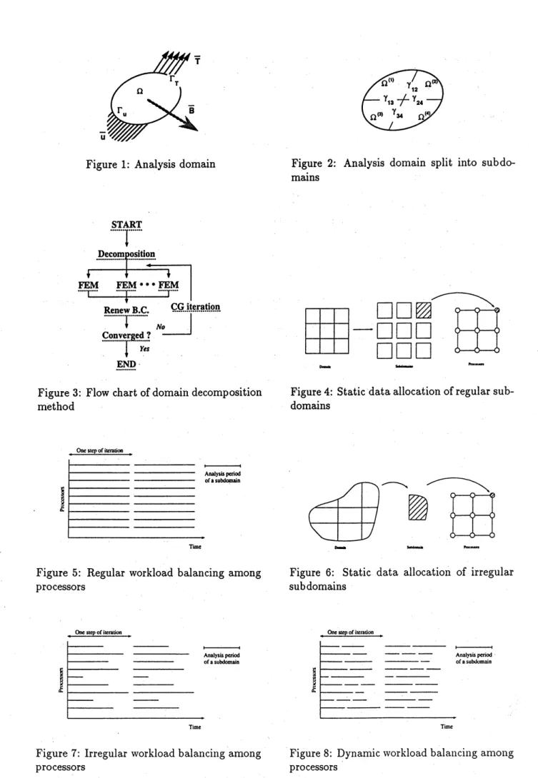
The present DDM is summarized in the following. To explainits theory, let us consider an elastic

problem concerning a domain $\Omega$, as shown in Figure 1. Here, $\overline{\mathrm{T}}$ is the traction force applied on

the boundary $\Gamma_{\mathrm{T}},$

$\overline{\mathrm{B}}$

thebody force appliedin the domain $\Omega,$ and$\overline{\mathrm{u}}$the prescribed displacement

on the boundary $\mathrm{r}_{\mathrm{u}}$.

Fundamental equations of this elastic problem are summarized in an infinitesimal displacenlent

mode as follows: _,. $r$

$\epsilon_{ij}=\frac{1}{2}(u_{i,j}+u_{j,i})$ in $\Omega$ (1)

$\sigma_{ij}=\overline{C}_{ijmn}mn^{\mathcal{E}}$ in $\Omega$ (2)

$\sigma_{ij}\nu_{ji}-\overline{T}=0$ $u_{i}=\overline{u}_{i}$ on $\mathrm{r}_{\mathrm{T}}$ on $\mathrm{r}_{\mathrm{u}}$ (4) (5)

where $i,j$ take the value 1 to 3, $u_{i}$ is

a

$C_{ijmn}$ a coefficient tensor of the Hooke’s law and $\nu_{j}$ an outer normal vector on the boundary $\Gamma$,

respectively. $()_{j}$, denotes the first order derivative with respect to thecoordinate $x_{j}$.

The above variationalform isequivalent to the followingminimizationproblem which finds the

displacementfunct\’ion $u$ which is astationary point of the energy functional:

$J(v)= \frac{1}{2}\int_{\Omega}\sigma_{ij}\epsilon_{ij}d\Omega-\int_{\Omega}\overline{B}_{i}v_{i}d\Omega-\int_{\Gamma}\overline{T}_{i}v_{i}d\mathrm{r}$ (6)

As shown in Figure 2, after dividing domain $\Omega$ into $N_{d}$ subdomains, $(\Omega^{(\dot{d})})_{1\leq}d\leq N_{\mathrm{d}}$ with

$\gamma_{pq}$

being the interface between $\Omega^{(p)}$ and $\Omega^{(q)}$, solving the above problem is equivalent to finding the

displacement functions $u^{(d)}$ which are stationary points of the energy functional:

$J’(v^{(1)}, \ldots, v^{(N_{d})(1})=’\dot{J})(v^{(1)})+J^{(}2)(v^{(})2)+\cdots+J^{(N_{d})(}(\dot{v})N_{d})$ ₍₇₎

with additional conditions on the interface boundary $\gamma_{pq}$:

$u^{(\mathrm{p})}=u^{(q})$ on

$\gamma_{pq}$ (8)

$\sigma_{ij}^{(p)}\nu^{(\mathrm{p}}jij)+\sigma^{(}\nu=0q)i(q)$ on

$\gamma_{\mathrm{p}q}$ (9)

where the superscripts $()^{(d)}$ designate variable defined in the subdomains $\Omega^{(d)}$

.

Depending on the treatment of additional interface boundary conditions of equations (8) and

(9), the following two approaches are available : In the first approach, equation (8) is satisfied

exactly, while equation (9) is approximately satisfied, and vice versa in the second approach.

Although both theapproachesare valid in principle, the first formulation involvesfullyNeumann

type calculations, which often generates floating domains that do not have enough prescribed

displacements to eliminate the local rigidbody modes. The second approach is thus thought to be

more appropriate.

With the use of a Lagrange nlultiplier method, solving the equation (7) with the subsidiary

condition (9) is equivalent to finding the saddle-point of the $\mathrm{L}\mathrm{a}\mathrm{g}_{\Gamma \mathrm{a}}11\mathrm{g}\mathrm{i}\mathrm{a}\mathrm{n}$ functional:

$\mathcal{L}(v^{()},., v^{(N_{d}}1..),(1)\mu,$ _{$\ldots,\mu^{()})N.=\sum^{N}J(d)(v^{()})+\sum_{pd,q}^{N}d\int_{\gamma}\mathrm{d}d,$}

$v\mathrm{p}q\mu\tau C(v(p)(q))d\gamma$ (10)

where

$c(v^{(\mathrm{p})},v)(q)=\sigma\nu^{(p}+i\mathrm{j}j\sigma(p))i(ji^{q}q)_{\nu^{()}}$ (11)

and$N_{:}$ is total d.o.f. on interface

$\gamma_{pq}$. The above problemcan be equivalently converted tofinding

the displacement functions $u^{(d)}$ and the interface Lagrange multipliers $\lambda^{(i)}$ that satisfy:

$\mathcal{L}(u^{(1)}, \ldots, u(N_{d}),(1):))\mu,$$:..,\mu^{(N}$ $\leq$

$\mathcal{L}(u^{(1)},’.\cdot.\cdot.\cdot,’ u^{()}\mathrm{d},’\lambda^{(1})v(N_{d})N\lambda^{()}1,’.\cdot.\cdot.\cdot,’\lambda\lambda(N..\cdot)))(N.)$ (12)

$\leq$ $\mathcal{L}(v^{(1)}$

for any admissible $(v^{(d)})_{1\leq}d\leq N_{d}$ and $(\mu^{(i)})_{1<i}<N.\cdot$

We can solve this saddle-point problem ($\overline{1}2\overline{)}$bya saddle-pointsolversuch as Uzawa’s$\mathrm{a}_{0}\mathrm{r}\mathrm{i}\mathrm{t}\mathrm{h}\mathrm{n}1$

or its CG variants. Let us describe the CG methodto solve the equation (12) in next section.

2.’2

Conjugate

Gradient

Algorithm

for

DDM

Defining the positive definite and symmetric operator $A$:

where

$u^{(\mathrm{P})}(\mu)=\mu^{(}q)(\mu)=\mu^{(i})$ on

$\gamma_{pq}$ (14)

the CG algorithm for solving equation (12) is summarized as follows:

Step $0$: Initialization $\mu^{(i)^{0}}$ : arbitrarilygiven (15) $g^{(i)^{0}}$ $=$ $A\mu^{(i)^{0}}$ (16) $w^{(i)^{0}}$ $=$ $g^{(i)^{0}}$ (17) The $g^{(i)^{0}}$

of equation (16) is obtained from the traction forces on $\gamma_{pq}$ which are calculated by

solving equations (1)$-(5)$ in each subdomains with the followingconstraint:

$u^{(p)}=u^{(q)}=\mu^{(i)^{0}}$ _on

$\gamma_{\mathrm{p}q}$ (18)

Step 1: Steepest descent

$\mu^{(i)^{n+1}}=\mu-(i)n\rho^{n}w(i)n$ ₍₁₉₎

where

$\sum^{N}.\cdot g^{(i)}ng^{(i)}n$

$\rho^{n}=.\cdot\frac{i}{N}$ (20)

$\sum_{:}w^{()^{n}}Aiw^{(}i)^{n}$

Step 2: Calculation ofthe new descent direction

$g^{(i)^{n+1}}=g-(i)^{nn}\rho^{n}Aw^{(i})$ ₍₂₁₎ $w^{(i)^{n+1}}=g^{(i)^{n+n}}1+\kappa wn(i)$ ₍₂₂₎ where $\sum^{N}.\cdot g^{(i)}gn+1(i)n+1$ $\kappa=.\cdot\frac{i}{N}$ (23) $\sum_{;}gg(i)^{n}(i)n$

The $Aw^{(i)^{n}}$ of equations (20) and (21) is obtained

from the traction forces on $\gamma_{pq}$ which are

calculated bysolving the following equations:

$\sigma_{ij,j}(d)=0$ in $\Omega^{(d)}$ (24)

$\sigma_{ij}(d)\nu j^{(d})=0$ on $\mathrm{r}_{\mathrm{T}^{(d)}}$ (25)

$u_{i}^{(d)}=0$ on$\mathrm{r}_{\mathrm{u}^{(d)}}$ (26)

$u_{i}(d)=wn$

on.

Step 3: Judgment ofconvergence

If$\mu^{(i)^{n}}$ has not converged yet, return to Step 1 by setting

$n$ to be $n+1$. Here the convergence

criterion is defined as:

$\frac{\max_{i}|g^{()^{n}}|i}{\max_{\dot{\iota}}|g^{(i)^{0}}|}<Err$ (28)

in which the $\mathrm{n}\mathrm{u}\mathrm{a}_{d}\mathrm{x}\mathrm{i}\mathrm{m}\mathrm{u}\mathrm{m}$ component of force imbalance along the interface boundary, i.e. residual

The flow chart of the present DDM algorithmisillustrated in Figure 3. It should be noted here

that the finite element analysis of each subdomain can be performed without any data

communi-cation among subdomains. Namely, the finite element analyses of subdomains can be performed

in parallel, once the displacement values on the inter-subdomain boundaries are given. Since the

workload foreach finite element calculation is much larger than those of other tasks including data

communication and modificationofboundary values, the so-called overhead due to parallel

calcu-lation is estimated to be verysmall. In addition, owing to thedecomposition ofa large scale finite

element system into a number of smaller sub-systems, only small computationstorage is needed

for each finite element calculation.

2.3

Preconditioning

for CG

In matrix formulation, problem (6) are given by:

$I\mathrm{i}^{r}u=f$ (29)

where $I\mathrm{i}^{r},$$u$, and$f$arerespectivelythestiffnessmatrix, the displacement vectorand$\mathrm{t}1_{1}\mathrm{e}$force vector

associated with the finite element discretization of$\Omega$.

For each subdomain problems of equations (24)$-(27)$, the matrix formulations are written as:

$I\mathrm{i}^{r}(d)u=(d)f(d),$ $d=1,2,$

$\ldots,$$N_{d}$ (30)

Let us use the $i$ and $b$ subscripts to designate internal and interface boundary d.o.f. and

if the

internal d.o.f. first and the interface boundary d.o.f. are numbered last, equation (30) can be

written as:

$[I\mathrm{i}_{ib}’I\mathrm{i}^{\prime(d)}(d)^{T}ii$ $Ii_{bb}I\zeta_{i,(d)}^{()},bd][u_{\iota^{d}}^{()}u_{i}^{(d)}]=[f_{b}^{(d}f_{i}^{(d)})]$ (31)

that is:

$Ii_{ii}^{\prime()}u_{i}^{()}dd+I\mathrm{i}_{ib}^{r}u_{b}^{()}(d)d$

$=$ $f_{i}^{(d)}$ (32) $I\mathrm{i}_{i\iota^{d)}i}u^{(}’(\tau d)’+I\mathrm{i}_{b\iota b}(d)_{u^{()}}d$

$=$ $f_{b}^{(d)}$ (33)

Fromequation (32):

$u_{i}=I(d)(di’ii)^{-1}(f_{i}(d)-IC_{i}(d)d))bu^{(}b$ ₍₃₄₎

From equations (33) and (34):

$(Ii_{bb}^{\prime(d}-)’(Ii_{i})dd))u_{b}(d))-IbI\iota^{\nearrow(d)^{-1}}\tau\tau(\mathrm{f}_{i}d\rangle I\zeta^{(d})-1iiI_{\dot{1}^{r(}}ibf_{b}^{(d}=biif_{i}(d)$

(35)

Considering the condition (24), equation (35) is written as:

$S(d)u_{b}(d)=f_{b}(d)$ ₍₃₆₎

where

$S^{(d)}=I\mathrm{i}_{bb}^{r()}d-I\mathrm{i}I’(d)ib\tau-1\mathrm{i}^{\prime(}ii\mathrm{A}_{i}^{(d)}bd)$,

(37)

$S^{(d)}$ is known as the local Schur

conuplement [21].

Now the operator $A$ofequations (20) and (21) is written as:

$A= \sum_{d}^{N_{\mathrm{d}}}B(d)s^{(d})B(d)^{T}$ (38)

where $B^{(d)}$ isa booleansymbolic

matrix which localizes a internal quantity totheinterface

For the above operator, a good preconditioner $P[22]$ can be constructed by assembling the

primal subdomainoperators as follows:

$P^{-1}= \sum_{d}^{N}Bd(d)B^{(d)^{T}}$ (39)

and it’s lumped preconditioner $P’$ is advocated in [23], that is:

$P’-1= \sum BNdd(d)B^{(d)^{T}}$ (40)

Thispreconditioner does not require anyadditional storage and involves only matrix-vector

prod-ucts ofsizes equal to the interface.

3

Implementation

on

MPP

As mentioned in the previous section, a large granularity oftasks can be obtained through the

DDM. To achieve high performance ofparallel algorithms, _{a technique to balance workload well}

among processors _{is demanded.}

With aSIMDtype of MPP,in orderto do so, we mustdivideadomainofconcernandprovideand

a uniform distribution with data to all processors in aregular fashion, although for a complicated

problem, it isnot easy.

To keep the load balance for an irregular decomposition problemsuch as a complicated nlodel,

dynamic _{data allocation, which can be performed by MIMD type of MPP, is desirable. With}

SIMD type of MPP, only data is distributed among _{processors, while with MIMD type ofMPP,}

instructions can be also distributed, that is, it can performmore advancedor complicated parallel

technique such as the dynamic _{data allocation.}

This fact thus motivated us to use _{the MIMD type of MPP with dynamic data allocation}

technique, and in addition for a large size problem, to avoid a limitation $\mathrm{f}\mathrm{r}\mathrm{o}\ln$ the memory size

of eachprocessors, the hierarchical _{data management technique is developed and implemented on}

MPP.

3.1

Data

Allocation

In each sub structuring or domain decomposition method, a physical problem, i.e. a domain

to be analyzed, _{is fictitiously divided into a number of subdomains. There are two approaches}

in allocating parallel tasks, i.e. calculations of subdomains, on multiple processors. The first

approach is_{the so-called “Static Workload Balancing” and the second isthe “Dynamic Workload}

Balancing”.

In _{static workload balancing, task allocation is performed a prioriconsidering workload balance}

among processors.

For simplicity, let us consider a problem which is divided into nine subdomains and allocated

to nine processors as shown in Figure 4. _{Considering how to allocate the divided data to each}

processor, a simple _{idea allows one subdomain data to be allocated to one processor when the}

nunlbers of subdomains and processors coincide. Therefore, _{in static workload balancing, it is}

important to divide domain into the same number ofsubdomains with processors.

With this nuethod, when all subdomain’s data are equal in size and the abilities of all the

processors are equivalent, all processors can start and end the analysis of each subdomain at the

same time and then change needed data among processors and start the next iteration step. In

such’a case, as shown in Figure5 wherein the vertical and horizontal axes denotes $\mathrm{t}\mathrm{l}\mathrm{l}\mathrm{e}$ number of

processors and $\mathrm{t}\mathrm{i}\mathrm{n}\mathrm{l}\mathrm{e}$,

respectively, well workload balancingcan be obtained easily.

Such a static workload balancingprocess iseasy to implement when the $\mathrm{d}_{01}1\mathrm{u}\mathrm{a}\mathrm{i}\mathrm{n}$ can be divided

regularlyinto the same number ofsubdomains with processors on aparallel computer which have

well when the geometry of the domain is complicated oreachprocessorhas a different performance

as can be seen in aclustered of different workstations.

When each size of subdomains are irregular (Figure 6) or processor’s abilities are different,

workload balance can not be obtainedsimilarly to the above case and it is getting lack of balance

as shown in Figure 7.

To handle this problem, another technique is needed to allocate the task to processors well,

which is so-called the dynamic workload balancingtechnique, and is described as follows.

In dynamic workload balancing, task allocation among processors is performed automatically

and dynamically during calculation.

Foran irregular decomposition problem, it isclearthatallocatingone subdomaintoone processor

can not obtain well workload balance as shown in Figure 7.

By combiningsmall and largesubdomains for each processor, the total workload balance can be

attained well as shown in Figure 8,

When the calculation time of each subdomain can be estimated prior to the calculation, task

allocation canbe performed beforehand statically,but usually it isnot easy toestimate accurately

and sometime it is changed during calculation. Therefore, to perform such an allocation, the

dynamic allocation is needed.

In dynamic allocation, data ofanother subdomain is provided as soon as the analysis ofone

sub-domainis finished. Anefficient workload is thus obtained if the whole domain is decolllp into a

large number of subdomains in comparisontothe number of processorsIn Figure8, twentydomains

are analyzed with nine processors where each processor deals with two or three subdolnains.

To take advantage of such dynamic workload balancing, the parallel finite element algorithnl

described in chapter 2 isimplemented on the MIMD type of MPP.

3.2

Roles

among

Processors

To implement the DDM which incorporates the dynamic workload balancing on the MIMD type

of MPP, we have to provide some roles to each processors. To allocate the data of$\mathrm{s}\mathrm{u}\mathrm{b}\mathrm{d}_{\mathrm{o}\mathrm{n}1}\mathrm{a}\mathrm{i}\mathrm{n}\mathrm{s}$

to processors, some processors have to manage data. That is, we need manager processors and

analyzerprocessors. With the MIMD of MPP, such tasks can be coordinated among processors.

Now, there are two types of management system, each consisting of either a manager and

analyzers set or one chief manager ‘Father-Child Model’, sonle managers $‘ \mathrm{G}\mathrm{r}\mathrm{a}\mathrm{n}\mathrm{d}_{-}\mathrm{F}\mathrm{a}\mathrm{t}\mathrm{h}\mathrm{e}\mathrm{r}$-Child

Model’ andanalyzers set. The latteris required fora large scale model which can notbe managed

by only one nlanager processor. These two types are described asfollows.

In ‘Father-Child Model’ system, one processor is set as a manager which is called ‘Father’ and

the others each as aanalyzerwhichiscalled ‘Child’. Figure 9 shows the schematic data flow among

processors ofthe present system. Theroleofthe ‘Father’ isto managedata and thatofthe ‘Child’

is to execute finite element analysis ofeach subdomain. The data flow anlong these two kinds of

processors are summarized asfollows.

The ‘Father’ reads nuesh data which is previously divided into some subdonlains and prepares

initial values onthe interface boundaries. After reading data froma disk ‘Father’ provides

subdo-main’s data to anyidling tChild’.

Now, any ‘Child’ can receive any subdomain’s data to reduce the idling time. As mentioned

in previous section , if subdomain’s data which are not of regular size are allocated to ‘Child’s

statically, some ‘Child’s have to wait until other ‘Child’ which is allocated to a larger subdonlain

complete the analysis of the subdomain. To handle this problem, in this $\mathrm{s}\mathrm{y}\mathrm{s}\mathrm{t}\mathrm{e}\mathrm{l}\mathrm{n}$, the ‘Child’

allocated to a smaller subdomain can get the next unsolved subdomain’s data as soon as the

previous analysis is over.

The ‘Child’whichreceives $\mathrm{s}\mathrm{u}\mathrm{b}\mathrm{d}_{0}1\mathrm{n}\mathrm{a}\mathrm{i}\mathrm{n}’ \mathrm{s}$data froma ‘Father’ executes thefinite element analysis

of.’

results ofthesubdomains, the ‘Fatller’ adjusts thevalues on the interface boulldaries so as to hold

the balance among subdomains. These operations are iterateduntil the convergence is achieved.

Figures 10 and 11 show the flow chart of ‘Father’ and ‘Child’ processors, respectively. Owing to

the processors dynamically as well as automatically.

In the previous system, all the data is first readby one ‘Father’ processor. Since in the case of

largescaleproblem, the data exceeds oneprocessor’s memory,thesystem obviouslyhas a limitation

in analysis in terms ofits memory size. To handle this problem, in (Grand-Father-Child _Model’

system, one processor is set as a chief manager which is termed ‘Grand’, some processors as a

nuanager termed ‘Father’ and the others as a analyzer termed ‘Child’.

Figure 12 shows the schematic data flow among processors of the present system. The role of

the ‘Grand’ is tomanagevaluesonthe interface boundaries andstatus of‘Father’ processors, that

of the ‘Father’ is to store and manage data while (Child’ _{executes the finite element} analysis of

eachsubdomain. The data flow among these three kinds of processors are summarized as follows.

The ‘Grand’ prepares initial values on the interface boundaries. Each ‘Father’ reads the whole

mesh data previously divided into the same number of parts as ‘Father’s and each part data is

divided into some subdomains. After reading the data from a disk (Father’ _{provides subdomain}

data to anyidling ‘Child’. The ‘Child’ which receives subdomain’s data from a ‘Father’ executes

the finiteelement analysisofthe subdomain and after the analysissends its result to the (Father’.

Now, every ‘Child’ can receive any subdomain’s data in the same way as the previous method,

and communicate with any ‘Father’ to reduce the idling time. That is, ifone of ‘Father’s $1$₎$\mathrm{a}\mathrm{s}$

no data for analysis, ‘Child’ which previously received data from the ‘Father’ can ask to another

‘Father’ for more data. As long as the ‘Father’ has the data ofthe subdomain for analysis, any

‘Child’ keeps working without idling. After receiving all the results of subdomains, the ‘Father’

sends results of interface boundaries to the ‘Grand’. The ‘Grand’ then adjusts the values on the

interface boundaries so as to hold the balance among subdomains. These operations are iterated

until the convergence is achieved.

Owing to the present dataflow mechanism, the proposed system can avoid a limitation

of’prob-$\mathrm{l}\mathrm{e}\mathrm{m}’ \mathrm{s}$ size which depended upon the memorysize of the father processor, and the whole workload

ofanalysis can be well-balanced among all the processors dynamically as well asautomatically.

3.3

Hierarchical DDM

Ill this parallel DDM, as shown in Figure 3, calculation time is in proportionto the number of CG

iterations. In CG method, its iteration nunuber much depends on d.o.f. of problem, i.e. in this

case d.o.f. on interface boundary. As the number of subdomains escalates with the scale ofthe

problem, the calculation time increases simply as well as d.o.f. on interface boundary.

In CG method, there exists a limit ofd.o.f.) over which the iteration number increases rapidly.

The limit depends on the colnple.\ity of the problem; i.e. for a large scale and complex $\mathrm{p}\mathrm{r}\mathrm{o}\mathrm{b}\mathrm{l}\mathrm{e}\mathrm{l}\mathrm{n}$,

calculation time could be enormous. To reduce the CG iteration number, it is needed to divide

problem into a small number of subdomains to reduce d.o.f. on the interface boundary. Since the

size of each subdomaindependson the number ofsubdomains, decreasing the$\mathrm{s}\mathrm{u}\mathrm{b}\mathrm{d}\mathrm{o}\mathrm{n}$

)$\mathrm{a}\mathrm{i}\mathrm{n}’ \mathrm{s}$number

causes increase of the subdomain’s size. Each subdomain’s size is, however, restricted in terms of

the memorysize ofa processor which analyze the subdomain. To handle the above problem for a

large scale analysis, a hierarchical DDM is developed in this paper, as described in the following.

In thisnew method, awhole analysis domain is first divided into a numberoflarge subdomains

in a rough manner. To do this, the total d.o.f. on the interface boundary can be set small, but

each subdomain’s size is over the domain that can be analyzed with one processor. To analyze

each subdomain, each subdomain is divided hierarchically into a number ofsub-subdomains and

apply the DDM to each subdomain. It means, in each $\mathrm{s}\mathrm{u}\mathrm{b}\mathrm{d}_{0}\mathrm{n}\mathrm{l}\mathrm{a}\mathrm{i}\mathrm{n}$, FEM analysis is $\mathrm{p}\mathrm{e}\mathrm{r}\mathrm{f}_{\mathrm{o}\mathrm{r}}\mathrm{n}\mathrm{l}\mathrm{e}\mathrm{d}$

by the DDM with iterative calculation. After achieving convergence in allsubdomains, the values

on the interface boundaries of all the subdomains are adjusted untilthe convergence in the whole

domain is achieved.

Notwithstanding the double loop of CG iteration, the hierarchical division can decrease d.o.f.

on interface boundaryunder keeping all the subdomains small in size. The flow of the hierarchical

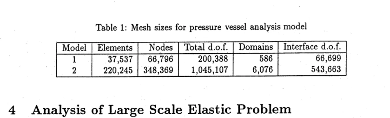
Table 1: Mesh sizes for pressure vessel analysis model

Model Elements Nodes Total d.o.f. Domains Interface d.o.f.

$1$ $2$ $37,537$ $220,245$ $66,796$ $348,369$ $200,388$ $1,045,107$ $586$ $6,076$ $66,699$ $543,663$

4

Analysis

of Large Scale

Elastic

Problem

For solvinga largescale model under the limitation ofmemory size, using very rough mesh which

cannot provide satisfied results or analyzing small part of the domain separately are the ways to

escape from its size problem. As supercomputers have enormous size of memory, this restriction

is getting removed and such a large scale model is becoming realistic for analysis though it was

considered impossible afew years ago. However, requirements for numerical simulation increases

much faster than the speedup of such supercomputers. The MPPs have the ability for large

scale analysismoregreatly than single processor computers, but such hardware needs appropriate

software.

With the present parallel FEM system, not only it can achieve high parallel performance, but

alsoit does not much depend on hardware. That is, it has ability to apply to any kind of parallel

computer with a high performance. As an application of the present system to a large scale

and complicated model, a whole pressure vessel with nozzles nuodel is analyzed in this chapter.

The problem is solved with some different ofparallel computer including workstation clusters to

estimate the robustness of the system.

4.1

Pressure

Model

The geometry of the model is defined and we assume that the inner surface of the model is under

pressure. The model was expressed by 10-noded tetrahedron elements with the density of lnesh

aroundnozzles being set higher than the other part. For this model,twosizesof niesh are generated,

models 1 and 2, sizes of which are listed in Table 1.

Each model is divided into subdomains with parameters listed in Table 1. This division is

determined from the capacity of the memory of ‘Child’ processor. To analyze the sanle $\mathrm{p}\mathrm{r}\mathrm{o}\mathrm{b}\mathrm{l}\mathrm{e}\mathrm{n}\mathrm{u}$ with different $\mathrm{C}\mathrm{o}\mathrm{n}\mathrm{l}\mathrm{P}^{\mathrm{u}\mathrm{t}\mathrm{r}\mathrm{s}}\mathrm{e}$, the menuory takes the value ofthe smallest processor’s $\mathrm{n}$)$\mathrm{e}\mathrm{n}\mathrm{u}\mathrm{o}\mathrm{r}\mathrm{y}$, which

amounts to 4 Mbytes memory. Since it is small, the number of divisions has become large which

causes a large nunlber of interface d.o.f.

In dividing into parts, the division number of parts depends on the memory size of ‘Father’

processor and since the number does not have effect on the number of CG iterations and since

sometimes it is not needed to divide into parts, i.e. in

case

available,it is set adaptiveto a computer to be used.

Figure 14 shows an example for amesh which is divided into 4 parts.

4.2

Comparison between Different

Conuputers

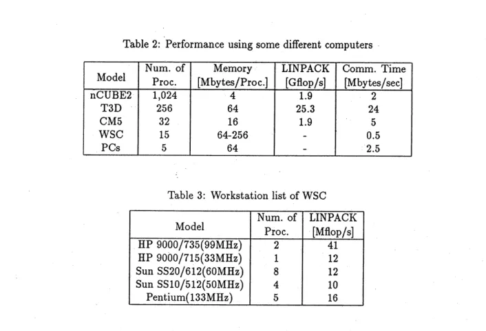
To compare performance between different computers, the model 1 was analyzedusing computers

listed in Table 2. The $\mathrm{n}\mathrm{C}\mathrm{U}\mathrm{B}\mathrm{E}2,$ $\mathrm{T}3\mathrm{D}$ and CM5 are commercial MPP, whereas WSC and PCs

are clustered computers substantially forming a parallel computer. The WSC is a workstation

cluster which consists of nine workstations having 15 processors wherein six workstations each

fine have two processors inside. The PCs are a personal computer cluster which consists of five

personal computers. These conlputers listed in Table 3 were connected through a network. The

WSC was connected through $10\mathrm{B}\mathrm{a}s\mathrm{e}5$ Ethernet, peak performance of which is 10 Mbps (Mega bit

per second), and the PCs are connected through $10\mathrm{B}\mathrm{a}\mathrm{s}\mathrm{e}\mathrm{T}$Fast-Ethernet whose performance is 10

$\mathrm{t}\mathrm{i}\mathrm{n})\mathrm{e}\mathrm{s}$higher than the WSC’s.

In Tables 2 and 3, as ayardstick of performance,it is referred to the LINPACK Benchmark [24]

conlmunica-Table 2: Performance using some different computers

Table 3: Workstation list of WSC

tion library was used and on the others PVM library [25] was utilized to communicate between

processors. .

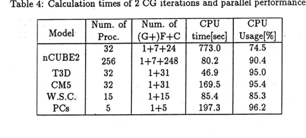
Calculation time of2 CG iterations on these computers and parallel performances

are

in Table 4. In the case of$\mathrm{n}\mathrm{C}\mathrm{U}\mathrm{B}\mathrm{E}2$, one processor was assigned as ‘Grand’, seven processors as

‘Father’ and the other processors, 24 or 248 as (Child’ _{considering small local memory size. For}

the other MPP’s cases, one processor was assigned as ‘Father’ and the other processors as ‘Child’.

On the WSC and $\mathrm{P}\mathrm{C}\mathrm{s}$, one processor assigned as ‘Father’ as well as ‘Child’ using the time sharing

system which permitted to be used by several tasks at thesame time and the other processors as

‘_Child’.

As a parallel performance, the rate ofCPU usage was used. The rate of CPU usage $R_{n}$ with $n$

processors is defined as follows:

$R_{n}= \frac{1}{n}\sum_{i}^{n}\frac{T_{w}^{(i}\circ rk)}{T_{wor}^{(i)}+^{\tau_{i}^{()}}kdil\mathrm{G}}$ (41)

where $T_{wotk}^{(i)}$ and $T_{id}^{(i)}\iota_{e}$ are the total time for working and idling of each

processor during the whole

computation,respectively. As shown in Table4, highparallel performances over 90 % are achieved

for all the cases except two cases, i.e. cases of $\mathrm{n}\mathrm{C}\mathrm{U}\mathrm{B}\mathrm{E}2$ with 32 processors and WSC. In the

former case, thereason is that number of ‘Father’sis too large compared with number of ‘Child’s.

Seeing CPU usage amongonly ‘Child’ processors, it achieved over99%. In the latter case, the low

performance result fromthe slow $\mathrm{c}\mathrm{o}\mathrm{l}\mathrm{n}\mathrm{m}\mathrm{u}\mathrm{n}\mathrm{i}\mathrm{C}\mathrm{a}\mathrm{t}\mathrm{i}_{\mathrm{o}\mathrm{n}}$ time using Ethernet.

4.3

Sorting

Technique

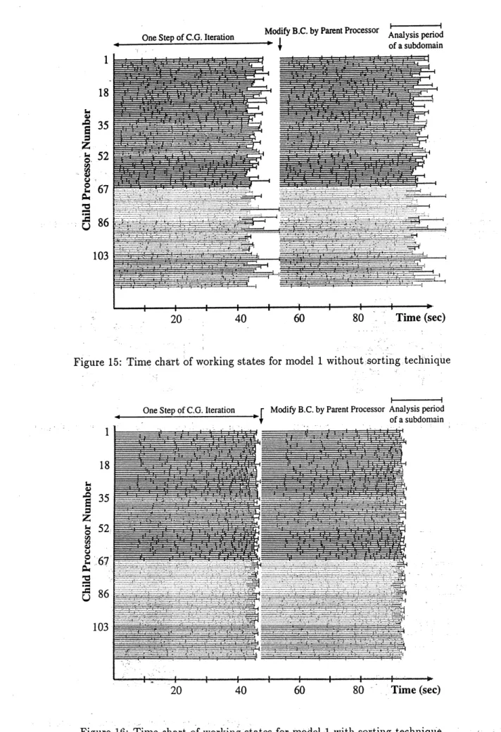
To demonstrate the dynamic allocation system described in section 3.1, the model 2 was solved

again with the $\mathrm{n}\mathrm{C}\mathrm{U}\mathrm{B}\mathrm{E}2$ consists of128 processors. In this

example, one processor was assigned as

‘Grand’, seven as ‘Father’ and 120 as (Child’.

’Figure 15 shows the time chart ofworking

_sta.tes

iterative steps of CG iterations. In this figure, the length of each horizontal bar indicates the

analysis period of asubdomainand the blanks indicate the idling timeof‘Child’processor waiting

subdomain’s data to analyze from ‘Father’ processor. The seven color means in which ‘Father’

Table4: Calculation times of 2 CG iterations and parallelperformances

magenta color (Father’. _{For example, No.l ‘Child’ is provided from magenta ‘Father’ and No.18}

(Child’ is from red _{’Father’,first.}

However, asdescribedin section3.2, the relation isjustadefaultset,i.e. any ‘Child’ can get data

from any ‘Father’. For example, No.1 (Child’ _{is provided from first} nine _{subdomains of magenta}

‘Father’,butwhen it finishes the ninthsubdomain,the magenta ‘Father’ can not provide next data

because he has no more unsolved data, so No.l ‘Child’ requires to another ‘Father’ and then can

get the next data from the blue ‘Father’.

In this figure, there is still a wide space of black which causes efficiency to be low. The reason

is that the subdomain which is finished to be analyzed last has a larger size. Sorting subdomains

datafromlargeto small, the larger subdomains can be analyzedinthe first period ofone iteration

step. Figure 16 shows the new time chart after sorting subdomain’s data. As shownin the figure,

it clearlydemonstrates that the work load balance among processors isfulfilled automaticallyand

$.\mathrm{d}$ynamically, thanks to thesorting technique.

In the model 1 case, one size ofeach subdomain is small enough $\mathrm{c}\dot{\mathrm{o}}$

mpared $\dot{\mathrm{w}}$

ith the total $\mathrm{t}\mathrm{i}\mathrm{n}$

)$\mathrm{e}$ ofeach iteration$\mathrm{s}\mathrm{t}\mathrm{e}\mathrm{p},$

$.\mathrm{e}\mathrm{V}\mathrm{e}\mathrm{n}$ without the sorting technique, it can perform with high efficiency.

4.4

Analysis of Pressure Vessel Model

For model 1, the$\mathrm{n}\mathrm{C}\mathrm{U}\mathrm{B}\mathrm{E}2$ consistsof 1,024 processors was used tosolve. As shownin Table 2, the memorysize $\mathrm{o}\mathrm{f}\mathrm{n}\mathrm{C}\sim \mathrm{U}\mathrm{B}\mathrm{E}2$is4 Mbytes and because of it, the model was divided into 25 parts to be

read by such processors. Therefore, one was assigned as ‘Grand’, 25 as ‘Father’ and the rest 998

as ‘Child’.

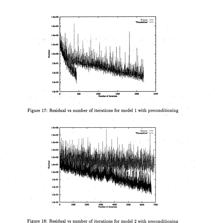
To estimate the convergence, the variations of the residual value, defined in equation (28),

against the number of the CG iterations of the two models 1 and 2 are shown in Figure 17

and 18, respectively. In each model, two cases are plotted, i.e. using normal CG algorithm

and preconditioning CG algorithm which is described in

_section.

in.

preconditioning technic is useful and necessary.

To check the convergence of aphysical value for this

modei,

has 71,022 d.o.f., was analyzed. Figures 19 and 20 show the variations ofthe residual value and

the displacement of one position which is on the inner surface of the vessel with respect to the

number of the CG iterations, respectively. As shown in these figures, despite the fact that the

residual values vibrate locally, the displacement value converges with the number ofiterations.

For model 1, over one million d.o.f. problem has been solved with 1,024 processors, 6,698

iterations, 182 hours and 96.5% parallelperformance,$\cdot$

5

Conclusions

TheparallelfiniteelementsystembasedontheDDM,which workson$\mathrm{a}..\mathrm{m}$

.assively

$\mathrm{p}\mathrm{a}\mathrm{r},\mathrm{a}\mathrm{l}\mathrm{l}\mathrm{e}\mathrm{l}$computer

were successfully developed in thepresent study.

Thissystemcan beappliedto severaltypesof parallelcomputersincluding clustered workstations

This system combined with preconditioning for CG wasapplied toa pressure vessel with nozzles

model with nonuniform mesh and irregular domain decomposition of over one milliond.o.f. and a

parallel performance ofover 90 with 1,024 CPUs was obtained.

References

[1] G.S.Almasi and A.Gottlieb, Highly parallelcomputing, The Benjamin $/Cummings$ Publishing Company (1994).

[2] BBN, ParaUel computingpast present and future, Technical report, BBNAdvanced Computers Inc.,

Cam-bridge, MA 11 (1990).

[3] L.H.Turcotte, A survey of softwareenvironmentsfor exploiting networkedcomputingresources, Engineering Research Center_for Computational Field Simulation (1993).

[4] C.Farhat and L.Crivelli, A generalapproachtononlinear FEcomputationsonshared-memory multiprocessors, Computer Methods in AppliedMechanics and Engineering72 (1989) 153-171.

[5] C.Farhatand E.Wilson, Anew finite elementconcurrentcomputerprogramar&itecture,International

Jour-nal_forNumerical Methods in Engineering 24 (1987)1771-1792.

[6] O.O.StoraasliandP.Bergan,Anonlinear substructuring methodfor concurrentprocessingcomputers,AIAA

Journal 25 (1987)871-876.

[7] C.Farhat, E.Wilsonand $\mathrm{G}.\mathrm{p}_{\mathrm{o}\mathrm{W}\mathrm{e}}\mathrm{U}$, Solutionoffinite element systems on concurrent

processing computers,

Engineering with Computers 2 (1987) 157-165.

[8] J.H.Hajjar and J.F.Abel, Parallel processingfor transientnonlinearstructural dynamics of$\mathrm{t}\mathrm{h}\mathrm{r}\mathrm{e}\mathrm{e}-\mathrm{d}\mathrm{i}\mathrm{m}\mathrm{e}\mathrm{n}\mathrm{s}\mathrm{i}\mathrm{o}\mathrm{n}\mathrm{a}\mathrm{l}\backslash$

framedstructuresusing domain decomposition, Computers andStructures30 (1988) 1237-1254.

[9] J.Hajjar and J.Abel,On theaccuracy ofsome$\mathrm{d}\mathrm{o}\mathrm{m}\mathrm{a}\mathrm{i}\mathrm{n}_{-}\mathrm{b}\mathrm{y}-\mathrm{d}\mathrm{o}\mathrm{m}\mathrm{a}\mathrm{i}\mathrm{n}$ algorithmsfor parallelprocessing

oftransient structuraldynamics, International Journal_forNumerical Methods in Engineering 28 (1989)1855-1874.

[10] _{1.S.Doltsinis and S.Noelting, Studies on}parauelprocessing forcoupled_{field problems, Computer Methods in} Applied _{Mechanics and Engineering}89 (1991) 497-521.

[11] R.Glowinski, O.V.Dinhand J.Periaux, Domaindecompositionmethods for nonlinearproblems in fluid dy-namics, Computer Methods inApplied Mechanics and Engineering40 (1983) 27-109.

[12] C.T.Sun and$1<.\mathrm{M}.\mathrm{M}\mathrm{a}\mathrm{o}$, A

$\mathrm{g}\mathrm{l}\mathrm{o}\mathrm{b}\mathrm{a}\mathrm{l}- 1\propto \mathrm{a}\iota$finite element method suitable forparallel computations, Computers

and Structures29 (1988)309-315.

[13] A.l$<.\mathrm{N}\mathrm{o}\mathrm{o}\mathrm{r}$and J.M.Peters, A partitioning

strategy forefficient nonlinearfiniteelement dynamic analysison

multiprocessorcomputers, Computers and Structures 31 (1989)795-810.

[14] R.Glowinski, G.H.Golub, G.A.Meurant and J.Periaux (eds), First internationalsymposium on domain dc-compositionmethods forpartialdifferentialequations, SIAM. Philadelphiar PA (1988).

[15]

$3- 9\mathrm{G}.\mathrm{Y}$

.agawa,

[16] J.C.LuoandM.B.Friedman, Implicit decompositionas a tool forsolvinglarge-scale structuralsystems in a

parallel environment, Computers and Structures35 (1990) 215-220.

[17] Y. ZhangandR.S.Harichandran,Implicitsubdommin integration_{for dynamic analysis of large-scale structural}

systems, Computer Methods inAppliedMechanics and Engineering 81 (1990) 57-70.

[18] G.Yagawa, N.Soneda and S.Yoshimura, A large scale finite element analysis using domain decomposition

method onparauel computer, Computers andStructures38 (1991)615-625.

[19] G.Yagawa, A.Yoshiok, N.Sonedaand S.Yoshimura, Aparallel_{finite element method with asupercomputer}

network, Computers andStructures47 (1993)407-418.

[20] G.Yagawaand

_R.Shio.ya,

decomposition, Computing systems in Engineering$4(4-6)$ _{(1994) 495-503.}

[21] P.E.Bjorstad andO.B.Widlund, Iterativemethods for thesolutionof ellipticproblemsonregionspartitioned

intosubstructures,SIAM J. Numer. Anal. 23(6) (1986) 1097-1120.

[22] J.Mandel,_{Balancing domain decomposition, Comm. Appl. Num. Meth. 9 (1993) 233-241.}

[23] C.Farhat and F.X.Roux, A method of finite element tearingand interconnectingand its parallel solution algorithm, International Journal_forNumerical Methods in Engineering32 (1991)1205-1227.

[24] J.J.Dongarra, Performanceofvariouscomputersusing standard linearequations software, Technical Report, Computer_{Science Department, University ofTennessee} $\mathrm{c}\mathrm{s}_{-}89-8\mathrm{s}$(1995).

[25] A.Beguelin, J.Dongarra, A.Geist, R.Mancheck and V.sunderam, A user’s guide to PVM : Parallel virtual machine, Technical Report, Mathematical Sciences Section, Oak Ridge National Laboratory $\mathrm{o}\mathrm{R}\mathrm{N}\mathrm{L}/\mathrm{T}\mathrm{M}-$

Figure 1: Analysis domain Figure 2: Analysis domain split into

subdo-mains

Figure 3: Flow chart of domain decomposition Figure 4: Static data allocation of regular

sub-method domains

Figure 5: Regular workload balancing among Figure 6: Static data allocation of irregular

processors $\mathrm{s}\mathrm{u}\mathrm{b}\mathrm{d}_{\mathrm{o}\mathrm{m}\mathrm{a}}\mathrm{i}\mathrm{n}\mathrm{S}$

Figure 7: Irregularworkload balancingamong Figure 8: Dynamic workload balancing among

Figure 9: Schematic data flow among

Father-Child processors Figure 10: Flow chart of Father processor

Figure 11: Flow

_chart.

o.

pro..

essor-

Figure 14: Pressure vessel model divided into

Figure 15: Tinie chart of working states for model 1 without $\mathrm{S}.\mathrm{o}\mathrm{r}\mathrm{t}\mathrm{i}\mathrm{n}\backslash \mathrm{g}\mathrm{t}\mathrm{e}\mathrm{c}_{\wedge}\mathrm{h}$nique

Figure 17: Residual vs number of iterations for model 1 with preconditioning

Figure 18: Residual vs number of iterations for model 2 with preconditioning

Figure 19: Residual vs number ofiterations Figure 20: $\mathrm{D}\mathrm{i}_{\mathrm{S}}\mathrm{p}\mathrm{l}\mathrm{a}\mathrm{c}\mathrm{e}\mathrm{n}\mathrm{l}\mathrm{e}\mathrm{n}\mathrm{t}$ vs number of itera-tions