Solutions to a Singular Diffusion Equation(Nonlinear Mathematical Problems in Industry)

(1)

Solutions to a Singular Diffusion Equation $\ovalbox{\tt\small REJECT}\ovalbox{\tt\small REJECT} \mathbb{H}^{1}I$

$\ovalbox{\tt\small REJECT} ae\not\equiv-$ $\not\in\ovalbox{\tt\small REJECT}\ovalbox{\tt\small REJECT}$

(Yun-Gang Chen)

(Yoshikazu Giga)

(Koh Sato)

\S 1.

Introduction

We consider the following equation

$u_{t}=|u_{x}|^{-0}u_{xx}$, $(t, x)\in(0,T)\cross(0,1)$ (El)

$u(t, 0)=u(t, 1)=0$, $t\in[0, T]$ (E2)

$u(0, x)=u_{0}(x),u_{0}(x)\geq 0,0<x<1$ (E3)

where $\alpha\geq 0$ and $u_{0}$ is a smooth function on $(0,1)$. We may recognize

this equation as a diffusion equation whose diffusion coefficient is $|u_{x}|^{-\alpha}$

.

So if there is a point where $u_{x}$ is close to $0$, then we can guess that

very strong diffusion would be$\backslash happen$ at that point. This is a simple

example of p-Laplace equations. We refer to [EDB] for general regularity properties of solutions.

If wedifferentiate both sides of(El)(withrespect to$x$), and set_{$v=u_{x}$}, then the equation would be described as follows

$v_{t}=c(|v|^{p-2}v)_{xx}$ (P)

where $p=2-a$ and $c$is acertain constant. The property of the equation

depends on $p$. If $p>2$, this equation is called porous medium equation which presents a model of the diffusion in $porou^{-}s$ media. In the case of

$1<p<2$

, the equation is called plasma equation since it was derived

from the model describing the behavior of the plasma in strong magnetic

field. The later case (which corresponds to the case of $0<\alpha<1$ in

(El)$)$, Berryman and Holland showed that all positive solution to the

equation (P) vanishes in finite time (i.e. $\exists t_{*}$ such that $v(t, \cdot)arrow 0$ as

$tarrow t_{*})$ under the Dirichlet boundary condition. Furthermore, the profile

of each solution tends to that of a certain separable solution as $tarrow t_{*}$

([B],[BHI]).

But those results on (P) can not be applied directly to our prob-lem. Because boundary coiiditions are different and another restriction

(2)

We first look for non-negative separable solutions of $(E1)-(E2)$ _{(\S 2),}

then we construct a stable difference scheme which approximates (El)

(\S 3). The result of the numerical experiment gives us a hint that the

solutions to $(E1)-(E3)$ also vanishes in finite time _(We shall prove this

fact in our forthcoming paper [OS]$)$. We apply a rescaling technique to the scheme to obtain more precise value of the vanishing time and the asymptotic profile of the solutions (\S 4).

\S 2.

Separable Solution

First, we look for a non-negative separable solution $u(t, x)=U(x)$ .

$T(t)$ of

$u_{t}|u_{x}|^{\alpha}=u_{xx}$ (2.1)

which is derived from (El), where $U(x)$ and $T(t)$ are assumed to be

non-negative $C^{2}$

functions.

Thus we get the following equations,

$T^{\alpha-1}(t)T’(\underline{t})=U^{-1}(x)|U’(x)|^{-\alpha}U’’(x)=-c(S)$

where $c>0$, since $U”(x)\leq 0$ can be obtained from $U(O)=U(1)=0$ and

$U\geq 0$.

Then we are led to the $follo\iota ving$ equations for $U(x)$ and $T(t)$

$T(t)^{\alpha-1}\cdot T’(t)=-c$ $(S1)$

$U”(x)=-cU(x)|U’(x)|^{\alpha}$. $(S2)$

Note if we assnme $\tilde{U}(x)=\beta U(x)$ and $\tilde{T}(t)=\beta^{-1}T(t)$ where $\beta$ is a

positive constant, then $U(x)T(t)=\tilde{U}(x)\tilde{T}(t)$ and

$\tilde{T}^{\alpha-1}(t)\tilde{T}’(t)=\tilde{U}^{-1}(x)|\tilde{U}’(x)|^{-\alpha}\tilde{U}’’(x)=-\beta^{-\alpha}c$.

Now, we may assume $c=1/\alpha$ without loss of generality. Then from

(Sl), we can easily see that the separable solution can be written as

follows

$u(t, x)=(t_{*}-t)^{1/\alpha}U(x)$

where $t_{*}>0$ is the vanishing time and $U(x)$ is asolution of the following

equation

$U”(x)=-[f(x)|U’(x)|^{\alpha}\underline{1},$

_{$U(x)>0,0<x<1$}

_(Dl)

$\alpha$

(3)

Thus, we can find $U(x)$ from (Dl), (D2) by the following way.

Proposition. Suppose $V(x)\geq 0$ satisfies the followingequations

$V”(x)=- \frac{1}{a}V(x)(V’(x))^{\alpha},$ _{$V’(x)\geq 0,0\leq x\leq 1/2$} (Vl)

$V(0)=0$ (V2)

$V’(1/2)=0$

.

(V3)

Then

$U(x)=\{\begin{array}{ll}V(x), 0\leq x\leq 1/2V(1-x), 1/2<x\leq 1\end{array}$

is a symmetric solution of (Dl), (D2).

Proof. Multiply both sides of (Vl) by $(V’(x))^{1-\alpha}$ and integrate them

from $0$ to _$x$. Then with astandard calculation, we can obtain the

follow-ing

$V’(x)=(V’(0)^{2-\alpha}-c_{\alpha}V(x)^{2})^{\frac{1}{2-\alpha}}$ (2.2)

where $c_{\alpha}= \frac{2-a}{2\alpha}$, and get

$V(x)=V’(0)^{1-\frac{\alpha}{2}}c_{\alpha}^{-\frac{1}{2}}W^{-1}(V’(0)^{\frac{\alpha}{2}}c^{\frac{1}{\alpha 2}}x)$.

Here $W^{-1}(x)$ is the inverse function of a non-decreasing function $W$ such

that

$W(y):= \int_{0}^{y}(1-s^{2})^{-\frac{1}{2-\alpha}d_{S}},$ $0\leq y\leq 1$

.

We note that the integral is convergent at $y=1$ and we put $W(1)=$

$M_{\alpha}(<\infty)$. But this solution only satisfies (Vl) and (V2) in a certain

interval not necessarily [0,1/2]. To satisfy (V3), $V$ has to attain its

maximum value at $x_{*}\leq 1/2$. We can express the $x_{*}$ at which $V(x)$

attains its maximum as follows

$x_{*}=V’(0)^{-\alpha/2}c_{\alpha}^{-1/2}M_{\alpha}$

.

And if $V’(O)$ is sufficiently large so that $x_{*}\leq 1/2$, we can write the

solution to $(V1)-(V3)$ as follows

(4)

Moreover, since $V’(x_{*})=V^{n}(x_{*})=0$ (because $\underline{d}_{W^{-1}(M)}=0$), we

$dx$

obtain $U(x)\in C^{2}(0,1)$. Obviously $U(x)$ satisfies (Dl) in (0,1/2) and

$U(x)$ satisfies (D2). Since the following equations

$\frac{d}{dx}V(1-x)=-V’(1-x),$ $\frac{d^{2}}{dx^{2}}V(1-x)=V^{u}(1-x)$

hold, $U(x)$ satisfies (Dl) also in (1/2,1).

Remark. $U(x)$ can be the profile of the separable solution of (El)$-(E2)$

(not (2.1)) only if $V(x)$ attains its unique maximum value at $x=1/2$.

We can show this, for instance, by using the theory of viscosity solution.

\S 3

Difference Scheme

To calculate the numerical solution of (E), we introduce a modified equation (E’) to overcome the difficulty in computing which occurs when

the value of the $u_{x}$ in (El) reaches $0$.

$u_{t}=|u_{x}^{2}+\delta|^{-\alpha/2}u_{xx}$, _{$(t, x)\in(0, T)\cross(0,1)$}, $(E’)$

This equation is an approximation of (El).

Now we introduce our difference scheme for (E’).

$\frac{u_{j}^{n+1}-u_{j}^{n}}{\tau}=\{(\frac{u_{j+1}^{n}-u_{j-1}^{n}}{\underline{9}h})^{2}+\delta\}^{-\alpha/2}\cdot\frac{u_{j+1}^{n+1}-2u_{j}^{n+1}+u_{j-1}^{n+1}}{h^{2}}$ , (3.1)

$u_{0}^{n}=u_{N}^{n}=0$, (3.2)

$u_{j}^{0}=u_{0}(jh)$, (3.3)

$1\leq j\leq N-1,$$n\geq$

. $0$,

where $N$ is the number of meshes, $h=1/N$ is the mesh size, $\tau>0$ is the

discrete time increment, and $u_{j}^{n}$ is the value ofthe numerical solution at

net point $(n\tau, jh)\in[0, T]\cross[0,1]$.

We can show that the difference scheme $(3.1)-(3.3)$ has $L^{\infty}$-stability.

Proposition. (Stability of the scheme) Let $\{u_{j}^{n}\}$ be the solution of

$(3.1)-(3.3)$. Then $\Vert u^{n}\Vert_{\infty}\leq\Vert u^{0}\Vert_{\infty}$ for $\forall n>0$ where

$\Vert u^{n}\Vert_{\infty}=\max j|u_{j}^{n}|$. Proof. We prove it by showing the following inequalities hold.

$\max ju_{j}^{n}\leq\max ju_{j}^{0}$ (3.4)

(5)

First, we rewrite (3.3) as follows

$-\lambda_{i}^{n}u_{j+1}^{n+1}+(1+2\lambda_{j}^{n})u_{j}^{n+1}-\lambda_{j}^{n}u_{j-1}^{n+1}=u_{j}^{n}$ where

$\lambda_{j}^{n}=\{(\frac{u_{j+1}^{n}-u_{j-1}^{n}}{2h})^{2}+\delta\}^{-\alpha/2}\cdot\frac{\tau}{h^{2}}$

.

Suppose for a fixed $n,$ $u_{m}^{n}= \max ju_{j}^{n}$

.

Then we can easily see that

$\sup_{j}u_{j}^{n}$ $=$

$u_{m}^{n}$

$\leq$ $-\lambda_{m}^{n-1}u_{m+1}^{n}+(1+2\lambda_{m}^{n-1})u$ $A$ $-\lambda_{m-1}^{n-1}u_{m-1}^{n}$

$=$ $u_{m}^{n-1}$

$\leq$

$\sup_{j}u_{j}^{n-1}$

and thus we can obtain (3.4). (3.5) can be shown in the same way.

Such a stability results is $pi^{\backslash }oved$ in [CGHH] for a singular equation

related to alevel set method for geometricevolutions in [CGG]. However

our equation (El) is not included in [CGHH].

\S 4

Rescaling

We computed the numerical solution for $(3.1)-(3.3)$ with several cases

of (El). From the computation, we can see that the solution to $(E1)-(E3)$

vanishes in finite time. So we tried to calculate $u(t, x)$ more accurately

especially when it vanishes, by using a “rescaling” approach for $u$ and

variable time increment $\tau$ in the following way.

Suppose

$v(t, x)=\Lambda\ell u(M^{-\alpha}t, x)$

.

(3.6)

It is easy to see that if $u(t, x)$ satisfies (2.1) then so does $v(t, x)$. So

we observe the value of $\Vert n^{n}\Vert_{\infty}$ at every time step. If the value become smaller than the given threshold (forinstance 1/2), then we rescale$u$ and

$\tau$ by (3.6) with $M=\Vert u^{n}\Vert_{\infty}^{-1}$ (i.e. multiply $u_{j}^{n}$ by $M$ and $\tau$ by $M^{-\alpha}$), and

continue to calculate the values of the solution for the next time step,

watchingin the same way. Thus, we can keep the value of$\delta$ small enough

compared with $u$, and $\tau$ would get smaller and smaller as $t_{n}$ gets close to the vanishing time.

(6)

In this way, we can obtain more accurate value of$u$ and its vanishing time numerically.

For semilinear heat equations, such a rescaling technique is applied in

[Ch].

\S 5.

Result of Numerical Experiment

We computed the asymptotic behavior of the solutions to (El)$-(E3)$

by the scheme $(3.1)-(3.3)$ with $h=1/64$ $(N=64),$ $\tau=2.5\cdot h^{2}$ and

$\delta=10^{-100}$. Note that we took 0.5 as a threshold of the rescaling, so

if $||u(t, \cdot)\Vert_{\infty}<1/2$ then rescaling would be done, so the $u(t, \cdot)$ would

be magnified and the value of $\tau$ becomes smaller. We present rescaled

profiles of$u$ for 3 different initial data with $\alpha=0.5$ (Figure 1 - 3). Each

figure contains its initial data $u_{0}$ (labeled $t0$), and rescaled profile of

$u(t, \cdot)$ (labeled tl-t5). The profile $tj$ is obtained by rescaling$j$ times of

original picture. The tiine $T_{i}$ ofthe profile $tj$ is displayed below the each

figures.

Initial data for each figures are as follows.

Figure 1. $u_{0}(x)=\sin\pi x$

Figure 2. $u_{0}(x)= \frac{64}{27}x^{3}(1-x)$

Figure 3. $u_{0}(x)= \frac{16}{15}\mu(\mu(x))$ where $\mu(x)\backslash =\frac{15}{4}x(1-x)$

.

The rescaled profile of numerical solutions to $(E1)-(E3)$ can be seen

to approach asymptotically to a certain profile.

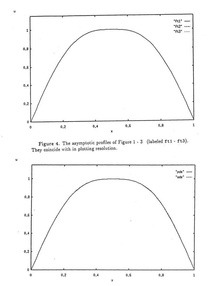
All computed asymptotic profiles of$u$ withdifferent initial data (plot-ted in Figure 1-3) coincide, at least in plotting resolution as shown in Figure 4.

Furthermore, the asymptotic profile (labeled pde) also coincide with

the $n\iota imerical$ solution for (Dl)$-(D2)$ (labeled ode) obtained by solving

(7)

Reference

[B] J.G.Berryman, Evolution

_of

a stable profile

_for

a class

_of

nonlinear

diffusion

equations with

_fixed

boundaries, Journal of Mathematical Physics, $18(1977),2108- 2115$.

[BHl] J.G.Berryman and C.J.Holland, Evolution

_of

a stable profile

_for

a class

_of

nonlinear

_diffusion

equations II, Journal of Mathematical Physics, $19(1978),2476- 2480$.

[Ch] Y.-G. Chen, Asymptotic behaviors

_of

blowing-up solutions

_for

_finite

difference

analogue

_of

$u_{t}=u_{xx}+u^{1+\alpha_{2}}$ J. Fac. Sci. Univ. Tokyo,

Sect. IA, Math. 33(1986), 541-574.

[CGG] Y.-G. Chen, Y. Giga and S.Goto, Uniqueness and existence

of

viscosity $solutio\eta^{\neg}$

’

of

generalized mean curvature

flow

equations,

Journal of Differential Geometry, 33$(1991),749- 786$

.

[CGHH] Y.-G. Chen, Y. Giga, T.Hitaka and M. Honma A stable

Differ-ence Scheme

_for

Computing Motion

_of

Level

_Surfaces

by the Mean

Curvature, preprint.

[EDB] E.DiBenedetto, Degenerate Parabolic Equations, Springer-Verlag,

1993.

[OS] M. Ohnuma and $I\backslash ^{\gamma}$. Sato, Remarks on Degenerate Parabolic

Equa-tions, in preparation.

Hokkaido Tokai

Universit}’

Sapporo 005, Japan and

Departnient of Mathematics Hokkaido University

(8)

$u$ $0$ 0.2 0.4 0.6 0.8 1 $x$ Figure 1. $T_{0}$ $=$ $0$ $T_{1}$ $=$

0.04516602

$T_{2}$ $=$

0.08173087

$T_{3}$ _$=$

0.1078698

$T_{4}$ _$=$

0.1262872

$T_{5}$ $=$

0.1392649

(9)

$u$ $0$ 0.2 _$0.4$ 0.6 0.8 1 $x$ Figure 2. $T_{0}$ _$=$ $0$ $T_{1}$ _$=$

0.02868652

$T_{2}$ $=$

0.06010765

$T_{3}$ _$=$

0.08589717

$T_{4}$ _$=$

0.1042887

$T_{5}$ _$=$ 0.1170933

(10)

$u$ $0$ 0.2 0.4 0.6 0.8 1 $x$ Figure 3. $T_{0}$ _$=$ $\mathfrak{a}$ $T_{1}$ _$=$

0.02624512

$T_{2}$ _$=$

0.06630449

$T_{3}$ _$=$

0.09247656

$T_{4}$ $=$

0.1109373

$T_{5}$ _$=$

0.1239462

(11)

$u$

$x$

Figure 4. The asymptotic $pi\cdot 0files$ of Figure 1 - 3 (labeled ftl - ft3).

They coincide with in plotting resolntion.

$u$

$0$ 0.2 $0.4$ 0.6 0.8 1

$x$

Figure 5. The asymplotic $pi\cdot 0files$ of $Figui\cdot e1- 3$ (labeled pde) and

rescaled profile of $sepai\cdot able$ solut$|on$ obtained by solving $(V1)-(\vee 3)$