近畿大学学術情報リポジトリ

全文

(1)Problems. in Three. Dimensional. Clouds. Simulation. in Star Formation. of. Process. Masayoshi. KIGUCHI. RIST, Kinki. University,. 5 77-8502,. of the Coil anse. Japan. (Received December 31, 2004) Abstract Numerical ing process, calculated. 1. procedure, is described.. by the nested. which. succeeds. The gravity. to simulate. is calculated. the three-dimensional by the multi-grid. method,. of gas in star form-. and the fluid dynamics. is. grid method.. Introduction. As found in the simulation of spherical collapse in star formation process(Masunaga, M. and Inutsuka, S., 2000), the first core with the radius of about 1 AU is formed, then second collapse is triggered by H2 dissociation. In its paper, radiation hydrodynamics is solved strictly and the radius and the luminosity of the primordial stars is calculated. In the real situation of the star formation, the assumption of spherical symmetry is not satisfied. The probability that the initial perturbation is in nearly spherical mode is very small, and the effect of the angular momentum is expected. We does not know the consequence of the asymmetry. In order to solve. 2. collapse. Grid. al., this difficulty. is managed. by the artful use of the. Lagrange mensional. scheme of the hydrodynamics. case, however, it is difficult. Lagrange. scheme. SPH method. directly. In three dito apply the. to the hydrodynamics.. does not have the ability to resolve. The the. process up to necessary to this problem. In this pager, therefore, we discuss the numerical problems to study the collapse problem focusing the hydrodynamics. The problems in radiative transfer is deferred to the future studies.. system. We apply the nested grid scheme ical process. these problems, we have to resolve the process from 104 AU to 10-3 AU. In the paper by Masunaga et.. up to necessary. to resolve. precision. the phys-. as follows:. AU. The ability of the PC in present. selectionof (N, L). We can take (N = 5, L = 12). We. dividethe cubic simulationbox to (2N)3cubic boxes. easily. with the same volume.. number. We call this grid system level. 0 grids. In the central part of the simulation. days limits the. box with. in reasonable is insufficient. calculation. time, but this grids. for the required. accuracy.. If. (1/2)3 of the total volume, we further divide each. we use parallel super-computer, we can take N = 8 easily and the required L is decreased to L = 15, but. cubes to 23 of same volume.. the L-nest. We call this grid system. level 1 grids. We recursively divide the central part up to level L. When we take N = 5, L = 18 level is necessary if we require the resolution up to 10-3. part can't. fit to the parallel. algorithm,. so. —9—. the limit of ability of L = 12 is same as the case of PC. We circumvent this limit by the refinement of the central part and the abandonment of the outer part in.

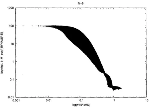
(2) the course of calculation.. 1 M® mass of spheroid. The number N can't be so small. Where the interval of grids changes to half, the numerical error of. in x-y direction and 2500 AU in z-direction. The abscissa is the logarithm of the distance from the center. calculation is induced by the change. If we demand that the error must be smaller than 3%, N> 5 is re-. log /x2 + y2+ z2 andtheordinateis the logarithm. quired. contact. the density is same for various distance r. We can read from this figure that the effect of improvement. Moreover, in order to resolve the shock or the discontinuity in each level, not so small N is. required. In figure 1, we show the initial stage of collapse. M. O C3 y. 0 L 0) O. O. U) N. O L OI O. of density. with axis length of 5000 AU. log p. As the morphology. is not spherical,. from N = 4 to N = 5 is large, but the improvement of. from N = 5 to N = 6 seems to be saturated..

(3) log(r/10^4AU) Figure. 3. Solving. Poisson. 1: Comparison. of the density distribution. for various. N. equation. The gravitygi is given by the Poisson equation:. point at each level is different point. We, therefore, calculate the potential value at finer grids from the a20 = 47-Gp, a one at coarser grid by the bi-linear interpolation forxiaxi mula and make the prolongation formula. From the adjoint condition, we make the restriction formula. 9i— =~(1) axi In the numerical calculation, the boundary condition for the Poisson equation must be imposed at where G is the gravitationalconstantand p is the den- finite distance. In initial, we put a uniform density sity. We can solve this equation by the multi-grid ellipsoid with axis length a1, a2, a3. In this case, the method (Hachbasch, 1985). The multi-gridmethod external potential is given by. is a hybrid iterativemethod. Using restrictionof potential cbto coarser grid systems and prolongation to finer grid system, long wavelength fluctuations are converged to zero, and using the Gauss-Seidel method, short wavelengthfluctuationsare converged to zero. We start to find the potential (/) level 0 by applying the multi-grid methods to the (2N)3 grids system. The density of level i is given by prolongating the density at level i + 1. After finding the solution in the level 0, we fix the boundary value of the potential for level 1, and proceed to the calculation in level 1. We continue this process to level N (Kiguchi, 2000). By the prolongation procedure of the density, the potential is found in each level up to the required accuracy, and we can neglect the effect of the finer level potential to the coarser level potential. The representation point of a cell is there at the center of the cell. This means that the representation. This potential as. is expressed. using the elliptic. integral.

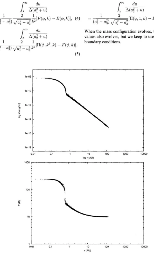
(4) When the mass values. also evolves,. boundary. Figure. 2 : The density. and temperature. distribution. configuration. evolves,. the boundary. but we keep to use this original. conditions.. for spherical. collapse. calculated. by 3-d code.

(5) 4. Hydro-dynamics. The basic equation momentum written as. where. of our problem. and the energy. state variables. is the mass, the whic h is. conservation,. the state Uoand proximate point,. the right cell has the state U1, the ap-. solution. is given as follows:. At left sonic. U are given by. At right sonic point,. for 1 < i < 3 in terms of the density p, the velocity and the internal. v. energy e, and the flux F is given by. At intersection. point,. for 1 < j < 3 in terms of the stress tensor, and the source term S is given by. where. where A is the volume heating rate. In inviscid case, which is our target, Cauchy stress tensor is cik = —p8iiand the thermal conduction flux is qi = 0 . In numerical simulation, we assume that the state valuables have a constant value in a grid cells with the representation point at the cell, and calculate the flux at the cell boundary. Using this approximate solution, the flux at the The accuracy of the time evolution and the width interface surface between these two cells is given by of a spatial cell are closely connected in the difference method for partial differential equations. When the width of a cell has the difference of factor two in neighboring cells, this difference easily leads to numerical instabilities such as spurious run-away to vanishing density in a cell. We tried various method (Toro, 1999) and found that Osher scheme is stable and simple, which is adequate for the nested grid sys- where tem. Osher scheme uses an approximate Riemann sovu lution which assumes there are three waves of contact discontinuity traveling with the velocity v, v c, In extreme case, there are possibilities that cso or csi where c is the sound velocity. When the left cell has becomes negative and Osher scheme fails. In this.

(6) case, all waves enter in the same cell, so that we can use complete upstream difference method. After updating the state using the flux term, we integrate the source term considering the equation as an ordinary differential equation which initial value is the updated. state. This method. corresponds. to the. variation of parameter method in inhomogeneous linear differential equations, i.e., this method is an approximate one in the case of non-linear it is strict in the linear case. In order to make the accuracy. equations,. of calculation. transfer in spherical case. We import the p-p relation from the spherical study and use the basic equation (7) inversely to determine the heating rate A. This p-p relation is as follows (Narita, 2002): At p < Pi = 10-15 g/ cm-3, the gas is in isothermal state,. p=mPHT=10K.Atp > p2= 10-1° gcm-3,the gas is in adiabatic is given. state, At pi < p < p2, the relation. but better. at the surface where neighboring cell width changes, one may think that fine cell should be embedded in the coarse cell and find the state in the fine cell by interpolation, but this method leads the calculation to an instability. The heating radiative problem.. transfer. rate A must be determined calculation,. Fortunately,. from the. but this is a difficult. we have the result of radiative. Using this relation, we can show that the first core with radius of about 1 AU is formed for the spherical collapse. of 1 M® using our three-dimensional. code. as shown in Figure 2.. References [1] Hackbasch,W., 1985,"MultigridMethodsand Applications",Springer-Verlag. [2] Kiguchi,M., 2000, Scienceand Technology,No. 12, 43. [3] Masunaga,H., Inutsuka, S., 2000, Ap. J., vol. 531, 350. [4] Toro,E. F., 1999,"Riemann Solversand NumericalMethodsfor Fluid Dynamics", Springer-Verlag. [5] Narita, S., 2002., Japan AstronomicalSocietyAutumn Assembly,p30..

(7)