Career Crisis? Impacts of Financial Shock on
the Entry-Level Labor Market: Evidence from
Thailand
著者
Machikita Tomohiro
権利
Copyrights 日本貿易振興機構(ジェトロ)アジア
経済研究所 / Institute of Developing
Economies, Japan External Trade Organization
(IDE-JETRO) http://www.ide.go.jp
journal or
publication title
IDE Discussion Paper
volume
83
year
2006-12-01
INSTITUTE OF DEVELOPING ECONOMIES
Discussion Papers are preliminary materials circulated
to stimulate discussions and critical comments
* Researcher, Regional Integration Studies Group, Inter-disciplinary Studies Center
IDE ([email protected])
DISCUSSION PAPER No. 83
Career Crisis? Impacts of Financial
Shock on the Entry-Level Labor
Market: Evidence from Thailand
Keywords: Crisis; Entry-Level labor Market; Job Loss; Treatment Effects; Thailand
JEL classification: C21, D83, J63, J64
The Institute of Developing Economies (IDE) is a semigovernmental,
nonpartisan, nonprofit research institute, founded in 1958. The Institute merged
with the Japan External Trade Organization (JETRO) on July 1, 1998.
The
Institute conducts basic and comprehensive studies on economic and related
affairs in all developing countries and regions, including Asia, the Middle East,
Africa, Latin America, Oceania, and Eastern Europe.
The views expressed in this publication are those of the author(s). Publication does not imply endorsement by the Institute of Developing Economies of any of the views expressed within.
INSTITUTE OF DEVELOPING ECONOMIES (IDE), JETRO 3-2-2, WAKABA, MIHAMA-KU, CHIBA-SHI
CHIBA 261-8545, JAPAN
©2006 by Institute of Developing Economies, JETRO
Abstract
We utilize Thailand's the financial crisis in 1997 as a natural experiment which
exogenously shifts labor demand. Convincing evidence from the Thailand Labor
Force Survey support the hypothesis that both employment opportunities and wages
shrunk for new entrants after the crisis. We find that workers who entered before the
crisis experienced job losses and wage losses. But these losses were smaller than
those of new entrants after the crisis. We also find that new entrants after the crisis
experienced a 10% reduction in the overtime wages compared to new entrants before
the crisis.
Career Crisis? Impacts of Financial Shock on the
Entry-Level Labor Market: Evidence from Thailand
∗Tomohiro Machikita†
Version Prepared in December 2006 - First Version in February 2005
Abstract
We utilize Thailand’s the financial crisis in 1997 as a natural experiment which exogenously shifts labor demand. Convincing evidence from the Thailand Labor Force Survey support the hypothesis that both employment opportunities and wages shrunk for new entrants after the crisis. We find that workers who entered before the crisis experienced job losses and wage losses. But these losses were smaller than those of new entrants after the crisis. We also find that new entrants after the crisis experienced a 10% reduction in the overtime wages compared to new entrants before the crisis.
JEL Classification Numbers: C21, D83, J63, J64
Keywords: Crisis; Entry-Level labor Market; Job Loss; Treatment Effects; Thailand
∗The author is indebted to Kenn Ariga for his generous support, advice, and encouragement. The author is also grateful
for the lively discussions with Naohito Abe, Yukiko Abe, Masayuki Doi, Yoshio Higuchi, Hidehiko Ichimura, Ryo Kambayashi, Daiji Kawaguchi, Yuichi Kimura, Yukihiko Kiyokawa, Anil Khosla, Kazuo Koike, Takashi Kurosaki, Masako Kurosawa, Kiyoshi Matsubara, Yasutomo Murasawa, Hisahiro Naito, Yoshihiko Nishiyama, Fumio Ohtake, Ryo Okui, Osamu Saito, Yuji Taka-batake, Makoto Watanabe, Futoshi Yamauchi, and Atsushi Yoshida. The author thanks the seminar participants at Institute of Economic Research Hitotsubashi Univerisity, Nagoya City, Nagoya, Institute of Statistical Research, and Applied Regional Science Conference, Japanese Economic Association. This project has not been carried out without their encouragement in the early stage of this writing. This research was supported by Grant-in-Aid for Young Scientist (No.18730159) of JSPS and a Grant-in-Aid for the 21st Century COE Program “Interfaces for Advanced Economic Analysis,” Kyoto University and “Re-search Unit for Statistical Analysis in Social Sciences,” Hitotsubashi University from the Ministry of Education, Culture, Sports, Science and Technology (MEXT).
†Corresponding address: Institute of Developing Economies (IDE-JETRO), 3-2-2 Wakaba, Mihama Chiba 261-8545, JAPAN.
1
Introduction
Does the financial crisis mean career crisis for new labor market entrants, youth, less educated groups during the period after a crisis? This paper examines the impacts of crisis on labor market outcomes utilizing the evidence that Thailand’s the financial crisis in the fall of 1997 exogenously shifted only the firm’s labor demand schedule. This exogenous and temporal aggregate shock is useful for identifying the impacts of the matching market conditions on employment, wages, and career dynamics subsequent to the financial crisis. This shock is also useful for identifying the complexity of the relative importance between returns to age (or to potential labor market experience) and years of schooling in the period after the crisis. To determine the causal effects of the financial crisis on aggregate labor market, we exclude not only the possibility of information problems in the job search and hiring process but also technological changes under the financial crisis. This paper does not consider the possibility of causal effects of financial crisis on frictional unemployment due to imperfect information on job and worker location. This paper also excludes the causal effects of financial crisis on structural unemployment due to mismatches between worker skills and firm technology. Exogenous aspects of financial crisis enable us to concentrate on cyclical unemployment due to voluntary unemployment involving worker transitions from declining industries to booming industries and involuntary unemployment like plant closings and demand shortages. Thanks to exogenous shifts in the labor demand, we can provide convincing evidence of the contribution of age and years of schooling to employment outcomes, i.e., labor force participation and wages. This paper is stimulated by seminal studies of economy-wide job training programs on individual outcomes. The benefit of using such experiments is shown in studies of the causal effects of government-provided training program on the duration of participants’ subsequent employment, unemployment spells, and earnings by Ham and LaLonde (1996) and by Heckman, Ichimura, Smith and Todd (1998). This paper is also stimulated by the studies on heterogeneity among displaced workers: Krueger and Summers (1988), Gibbons and Katz (1991), Gibbons and Katz (1992), Jacobson, LaLonde and Sullivan (1993), Neal (1995), Parent (2000), Kriechel (2003), and Dustmann and Meghir (2005). Recently, Rosenzweig and Wolpin (2000) and Angrist and Krueger (2001) summarize the benefits and shortcomings of natural experiments to compare the long-run outcome of treatment and control group using experimental or empirical data.
The empirical bottom line of this paper is based on the following works of empirical assessment of recent financial crisis on the labor market and households. One project focuses on the financial crisis in Indonesia. Another focuses on Argentina. Smith, Thomas, Frankenberg, Beegle and Teruel (2002) study the effects of the Indonesian financial crisis on wages and employment using household panel data from the Indonesian Family Life Survey (hereafter IFLS). They find that aggregate employment has remained robust because of industry-to-industry mobility. On the other hand, there was a dramatic decline of around 40% in the real hourly wages for urban workers. Frankenberg, Smith and Thomas (2003) argues the question of the household consumption response to the Indonesian the financial crisis. They show in full detail using IFLS,
that households reduced spending on semi-durables while maintaining expenditures on foods. Thomas, Beegle, Frankenberg, Sikoki, Strauss and Teruel (2004) extend the question of household response to the crisis to education expenditures for the next generation using IFLS. They find that household spending on education declined among the poorest households. They also find clear evidences of investment irreversibility in education. Educational spending was reduced among poor households with many young children, while there was a tendency to maintain education expenditures in poor households with older children. Finally, McKenzie (2004) examines the effects of the 2002 the financial crisis on households in Argentina and the urban labor market response, using panel data from an urban area survey. He finds that the crisis had a large aggregate effect, with 63% suffering a real income fall of 20% or more major job destruction.
Two testable implications are drawn from our theoretical framework: (1) selection tightens for new entrants in the period after the crisis because of lower labor demand due to the negative productivity shock; (2) the gap of employment opportunities and wages between new entrants in the period before and after the crisis persists. To examine the impacts of financial shock on the transition from school to work and subsequent career dynamics, we attempt to combine a search-theoretic framework with Mincer type wage regressions. We briefly explain our empirical implementation. First, we identify the treatment group and the control group in the face of the crisis using the individual record of “years of labor market experience” in our dataset in the period after the crisis. There are two treatment groups. The first, denoted by T1, is new entrants in the period after the crisis. This group seems to have difficulties finding jobs after entering the job search market due to the shock. The second treatment group, denoted by T2 is new entrants in the period before the crisis working in the period after the crisis. They were also affected by the unexpected shock. On the other hand, the control group, denoted C1, is new entrants in the period before the crisis working in the period before the crisis. The groups with subscript 1 (C1 and T1) are new entrants in the period before the crisis. We examine the impacts of financial shock on the entry-level job market by comparing the outcomes between the treatment and control groups. Secondly, we examines whether returns to age (or potential labor market experience) and years of schooling change or not during the period after the crisis. These parameters rule the labor market outcome.
From the viewpoint of our empirical implementation, using crisis as a natural experiment, it is diffi-cult for new entrants to find jobs in the period after a crisis. This evidence supports an aspect of the selection hypothesis. This is consistent with the statistical findings of Behrman, Deolalikar, Tinakorn and Chandoevwit (2000). We summarize our empirical results as follows: (1) the selection of the entry-level job market hypothesis is supported; (2) the gap of employment opportunities and wages between treatment (with shock) and control groups (without shock) increases over time. This shows the cohort effects of the financial crisis on new entrants. Evidence from our dataset, Thailand Labor Force Survey, supports the conclusion that both employment opportunities and wages shrunk for new entrants after the crisis. We find
that new entrants before the crisis also experienced job losses and wage losses. But these losses were smaller than those of new entrants after the crisis. We also find that new entrants after the crisis experienced a 10% reduction in the overtime wage level than new entrants before the crisis.
The structure of this paper is as followings. Next section 2 introduces the Thailand the financial crisis in the summer of 1997 as a natural experimental setting. Section 3 simply models our theoretical background to derive empirical hypotheses. Section 4 presents our data source, descriptive statistics, and key variables. Section 5 shows the impacts of crisis on the entry-level labor market. Our empirical results on the impacts of crisis on cohort effects for new entrants are shown in section 6. Concluding remarks are presented in the final section.
2
Estimating the Impacts of the Crisis for Career Determination
2.1 The Thai Financial Crisis of 1997
The financial crisis in Thailand in 1997 drastically changed labor market outcomes, labor force character-istics, and wage-profiles drastically. The crisis occurred in the early fall of 1997. It disturbed the labor market beginning in early 1998. It affected the unemployment rate, level of real wages, retention rate, and recruitment frequency through large-scale job destruction. Behrman and Tinakorn (2000) and Behrman et al. (2000) report and summarizes the labor market situations in those periods. They show the impacts of the crisis on the youth labor market and incumbent workers, percentage changes of employment, under-employed, unemployment, and the level of real average wages during the period before (1995-1996) and the period after the crisis (1998-1999). There was a particularly large negative shock for youth seeking employment. Real wages declined by approximately 10%. This paper formalizes the empirical evidences from previous literatures to create the treatment and control groups.
The financial crisis started from the financial market. It then spilled over from the financial sector to the manufacturing sector and commodity markets. It was an unexpected and exogenous shock for most incumbent workers and new entrants to the labor market. This paper takes Thailand’ the financial crisis as a natural experiment. From a statistical point of view, it is useful to focus on longitudinal evidence for the displacement of workers. We attempt to identify the contribution to the wage level of schooling, years of labor market experience, sector tenure, and firm specific tenure. Because this paper can not follow longitudinal evidence on individuals in the period before and after the crisis, we adopt another approach: seeking the difference of employment probability and wage level to identify the treatment group and control group using the exogenous shock.
2.2 Wage Profiles and Returns to Labor Market Experience
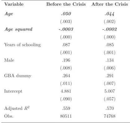
We compare the determinants of wage level in the period before the crisis with that in the period after the crisis. Firms, incumbent workers, and potential entrants faced demand shortages and job destruction in the period after the crisis. We assume that the distribution of unobserved individual abilities is not different between the two periods. Due to the labor demand shortages in the period after the crisis, it was difficult for new entrants to find employment and for current incumbents to move from job to job. Table 1 reveals clear contrasts in the contribution of age effects between the two periods. In short, estimates of the coefficient of age and square of age declined, while the effect of years of schooling was maintained in the period after the crisis. These results prompt us to search for the driving forces behind the two wage equations. There is a steep rise in the intercept in the period after the crisis. This can be explained by higher unobserved abilities of youth in the period after the crisis would be higher than that of youth in the period after the crisis. The two wage profiles have different curves. The wage profile in the period before the crisis draws a wide arc. The financial crisis of 1997 changes the arc of the curve. This is eloquently demonstrates the impact of the financial crisis on the labor market outcomes.
Before moving to the theoretical framework and formulating the empirical hypotheses, we will discuss returns to age in more detail. The important point to note is that the curve of returns to age becomes gentler after the crisis. This rule holds in all occupations, both white- and blue-collar. The two lines of the returns to age intersect around the age of 20 or 25 years. The line in the period before the crisis continues to decrease steeply after the intersection. On the other hand, the line of the period after the crisis continues to decrease moderately. This observation needs to be explained theoretically. Our hypotheses are induced by these structural changes on the wage equation.
2.3 Why Do Selected Entrants Experience Lower Paid Jobs over Time?
We present our empirical framework and testable hypothesis before beginning an empirical analysis. Our theory shows the causal effects of labor market conditions and match quality on individual outcomes. Our target is to estimate the impacts of entry-level labor demand conditions on employment outcomes. We consider the following relationship between individual outcomes and labor demand conditions:
yi = β0+ β1Di(p) + ui
Di(p) = α0+ α1Zi+ vi
where yi is employment outcome for new entrants which equals employment opportunities Ei and wages
log Wi. Di(p) is the entry-level labor market conditions, and is characterized by firm-specific productivity
level p, with ui being unobservable characteristics for econometricians (ability, match quality, or unmeasured
errors). Estimating the impacts of (entry-level) labor market conditions on the employment outcome is our target. This paper uses the evidence from Thailand’s the financial crisis in 1997 as a marker of aggregate
level of labor demand Zi of the variable of entry-level labor market condition Di(p). Thai financial crisis
of 1997 was an economy-wide shock and was exogenous for individual workers and potential workers (i.e., current students and graduates). These characteristics of the financial shock satisfy the two assumptions of strict exogeneity (E[Zi, ui] = 0) and the causal effects of Zi on Di(p).
Next, we can introduce the hypotheses to be examined. To do this, we focus on returns to years of labor market experience in the wage equation. Years of potential labor market experience reflect firm or industry specific human capital for each worker. If a worker is laid off during a crisis or quits her current match and moves to another firm or industry, her accumulated human capital would become obsolete. The decline of returns to experience on an aggregate level is supported by the job reallocation effect. If an incumbent is not laid off and does not quit during the crisis, it will be difficult for her to find entry into the tight market unless she has good luck or is highly capable. Selection becomes extremely tight for mass of new entrants. Only workers with good luck and high capability successfully enter and survive during the crisis. This selection effect pushes returns to labor market experience down. The decline of returns to experience of the aggregate level is also supported by the selection effect. Testing against the following hypotheses is a purely empirical exercise.
Crisis as an unexpected negative shock is an absolutely key assumption to do our empirical implementa-tion. By using a macroeconomic shock as a “natural experiment,” the model provides a new understanding of the relationship between on-the-job search and wages determination in the periods before and after the crisis. First, if incumbents tend with high probability to stay in office due to lower occurrence of job reallo-cations in the period after the crisis, then new entrants into the market will be severely restricted (by small size of search market).
Hypothesis 1 Selection at entry level tightens after a crisis. It is difficult for new entrants to be employed in the period after a crisis. Average productivity among newly employed workers is higher than that among newly employed workers in the period before a crisis.
Secondly, if a negative shock creates a large gap in employment probability between new entrants in the periods before and after the shock, the gap will tend to persist.
Hypothesis 2 The gap in employment probability and wage level persists between new entrants in the periods before and after a shock. New entrants experience lower paid jobs over time.
3
Data
3.1 The Thailand Labor Force Survey
The data source used in this paper is the Thailand Labor Force Survey (hereafter LFS), 1994-2000 by the The National Statistical Office (NSO) of Thailand. This individual-level data provides information on many individual characteristics: gender, structure of family, years of schooling, years of labor market experience, wages (or profit for self-employment household and profit for agricultural household), labor force status, migration status, hours and days of weekly work, occupation, industry, region, marital status; and employer characteristics: firm size, industry, and fringe benefits. LFS is carried occurs the four times per year. The first round is done in February, the dry season in Thailand. The third round is done in August, the monsoon (agricultural) season. We only use the third round survey in order to exclude seasonal labor migration in the dry season. The second and third rounds are done in May and November, respectively. Because LFS does not follow individuals from year to year, this study cannot be used to obtain information on labor mobility from the pre-crisis period to the post-crisis period. This study also uses pooled cross-sections from previous studies on aggregate labor market and urban immigration: Yamauchi (2002)’s study about migrants in the face of crisis in Bangkok, Kimura (2004)’s study on learning about one’s own ability by youth migrants to Bangkok.
The sample used in this paper comes not only from “Greater Bangkok Area” and other rural area; we use the sample from the entire Kingdom of Thailand, year 1994 to year 2000. We would like to mention the geographic characteristics. This paper adopts as GBA (Greater Bangkok Area) dummy variable which equals 1 if a province is included in the Bangkok metropolitan area. Nearly all industries and occupations tend to agglomerate in GBA. This classification using a regional dummy reflects the geographic distribution of industry and occupation in the face of crisis.
3.2 Definition and Construction of Treatment and Control Group
Let me summarize our data generation process for drawing strong power of identification. The details are shown in the section on empirical methodology. This paper constructs one unique variable on the basis of the information in the LFS, 1994-1996 and 1998-2000. This variable and some assumptions play important roles in identifying the treatment group and control group respectively. We construct a shock-dummy variable which identifies the treatment (new entrants in the period after the crisis) and control group (new entrants in the period before the crisis) using the information on the length of working life after graduation. We choose the variable “years of potential labor market experience” to examine the impacts of the crisis. We identify the treatment group and control group in the face of the crisis using the individual record of years of potential labor market experience. For the treatment group, the shock-dummy variable equals 1 if the worker had less than 1 year of experience in the survey year 1998, less than 2 years of experience in the
survey year 1999, and less than 3 years of experience in the survey year 2000. This group seems to have found it particularly difficult to get the job opportunities after entering the market due to unexpected exogenous shock. On the other hand, the control group has already entered the labor market in the period before the crisis.
Additionally, we set the “age at shock” dummy variable as equal to 1 if the individual’s age at crisis is
a. Finally, we also define the “years of schooling at shock” dummy variable as equal to 1 if the individual’s
years of schooling at the time of the crisis. We use those two dummy variables to check the parameter changes, i.e., returns to age and returns to years of schooling due to the crisis. The Treatment group is wage employed in the period after the crisis and the control group are those wage employed in the period before the crisis respectively.
3.3 Descriptive Analysis
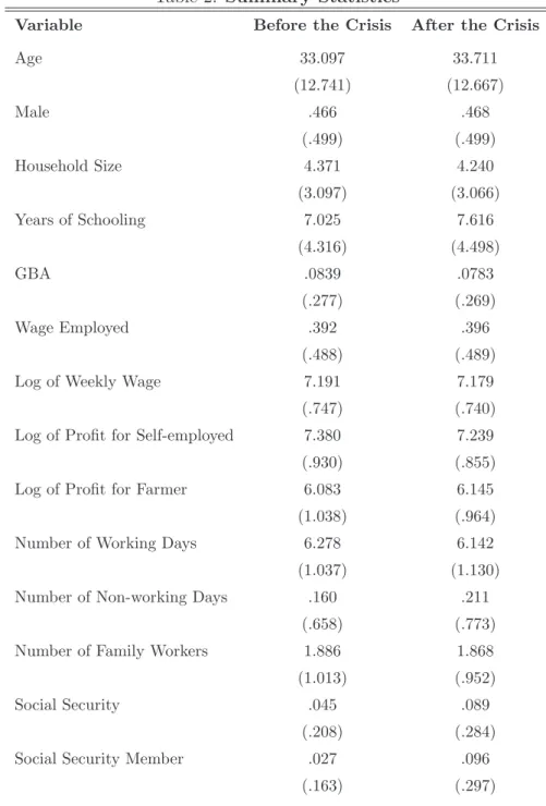
Table 2 shows the aggregate consequences of the crisis on the labor market. The variables are individual characteristics, industry categories, and occupation categories. Individual characteristics are age, gender, household size, years of schooling, living in Greater Bangkok Area, employment wage, log of weekly wage, log of profit for self-employment household, log of profit for agricultural household, number of working days per week, number non-working days per week, number of family workers in household, and social security status. We would like to emphasize four points regarding the changes of individual characteristics. First, urban population decreased in the period after the crisis, from 8.4% to 7.8%. Secondly, the log of weekly wage and log of profit for self-employment households decreased in the period after the crisis. On the other hand, the log of profit for agricultural households increased in the period after the crisis, from 6.08 to 6.14. Thirdly, number of working days decreased from 6.27 days per week to 6.14 days per week in the period after the crisis. Number of non-working days increased from 0.16 days per week to 0.21 days per week in the period after the crisis. However the standard deviations of both working and non-working days increased in the period after the crisis. Finally, social security status increased sharply in the period after the crisis. The percentage of workers belonging to firms with social security increased from 4.5% to 8.9% in the period after the crisis. The percentage of workers enrolled in social security also increased from 2.7% to 9.6%.
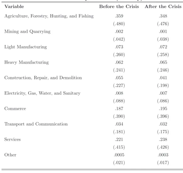
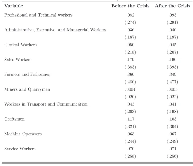
Industry features are summarized in Table 3. The highlight is decrease in the population in the construc-tion sector in the period after the crisis: from 5.5% to 4.1%. Heavy industry offered many job opportunities in the period after the crisis. Occupation features are summarized in Table 4. The population of craftsmen decreased in the period after the crisis: from 12% to 10%. The population of professional, technical, ad-ministrative, and managerial workers increased in the period after the crisis. The tables present an outline of the labor market in the period before and after the crisis. These tables show that aggregate employment opportunities seem to have remained stable between periods before and after the crisis. In this paper, we
look more carefully into the entry level.
We will focus attention now on the years of schooling and wage level. We decompose the aggregate level into simple occupation categories: white- and blue-collar simply. White-collar jobs cover occupations involv-ing professional, technical, administrative, executive, managerial, and clerical work. Blue-collar jobs cover occupations including sales, mining, transport and communication, production, and service. Agricultural workers are excluded from blue-collar workers. Both Table 5 and 6 present means and standard deviations for the main variables of our interests: years of schooling and log of weekly wages. Because of the showing clear contrast between the situations in the periods before and after the crisis, our sample in this summary is restricted by age and working status. Age is restricted to individuals from 13 to 59 years of age. Column 1 represents data for wage employees in the period before the crisis. Column 2 also shows data for wage employees in the period after the crisis. The table reports the data on years of schooling for two types of new entrants. Row 1 shows a steep rise of average years of schooling for wage employees in the period after the crisis. This reflects the increasing of educational attainment. Average years of schooling for white-collar workers, blue-collar workers, GBA workers, and rural area workers are also rose among those in the period after the crisis. This table shows the market selection and trend of educational attainment. Average years of schooling among the whole population and average years of schooling among wage employees 7.02 years and 8.63 years, respectively in the period before the crisis. Average years of schooling among the whole population and average years of schooling among wage employees were 7.61 years and 9.27 years in the period after the crisis. The increase of 0.39 years of schooling is a contribution of the aggregate trend during the periods. Market selection required an additional 1.61 years in the period before the crisis for wage employment and additional 1.66 years in the period after the crisis.
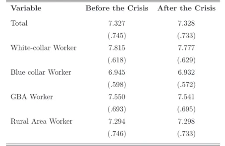
Table 6 shows the log of weekly wages for wage employees in the period before the crisis and for those employed in the period after the crisis. The wages for both white- and blue-collar workers decreased in the period after the crisis. But this was not a sharp decrease. The wage levels are quite similar between the two periods for GBA workers and rural workers. A rigorous analysis of the wage level will be given in the section on empirical results.
4
The Impacts of Crisis on the Entry-Level Labor Market
4.1 Empirical Methodology
We examine the effect of the crisis on employment for less-experienced workers, especially, for new entrants into the labor market. We assume that the crisis is an unexpected shock for every worker and every new graduate. No worker can expect how the shock will affect occupations, industries, and employment status. Our empirical methodology is quite similar to Duflo (2001)’s work on Indonesian school construction between
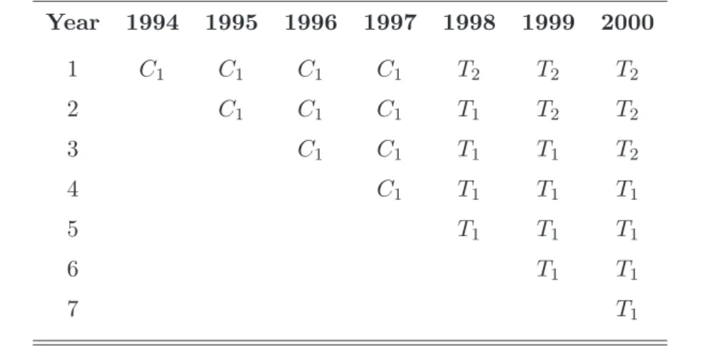
1973 and 1978 and Crepon and Kramarz (2002)’s study on the 1982 mandatory reduction of the workweek in France. Table 7 shows the dates of entry and years of potential labor market experiences for individual workers. Years of potential labor market experience means the age of an individual minus years of schooling completed in each survey year. New entrants into the labor market in the period before the crisis are briefly described in C1 (control ). The difference between the two types of new entrants is whether or not an individual is working in the period after the crisis. New entrants accumulate labor market experience every year. On the other hand, new entrants in the period before the crisis who were working in the period after the crisis are summarized as T1 (type1 treatment group). New entrants in the period after the crisis are also summarized as T2 (type 2 treatment group). We can observe that new entrants in 1994 had seven years of experience in the labor market by 2000 and new entrants in 1997 have four years of experience by 2000 from Table 7. An unexpected shock comes once in Thailand, in the summer and fall of 1997. We expect that it was more difficult for each T2 entrant to enter the labor market in the period during and after the crisis than compared to new entrants in the period before the crisis in groups C1 or T1.
Our empirical methodology requires the following two assumptions to be made in building an experimen-tal setting as suggested by Angrist, Imbens and Rubin (1996): random assignment and exclusion restrictions. Random assignment means that the crisis was an unexpected shock for incumbent workers and new entrants in labor market and that the treatment assignment T is random. The exclusion restriction means that each individual had no incentive to delay the timing of entry during the crisis period. This empirical methodol-ogy is straightforward, because the financial crisis as experiment took place at random. This randomization gives us a reduced-form approach for estimating the effect of the crisis on less-experienced workers. The reduced form effect of crisis can be shown here by comparing the mean labor market outcomes (employment and wages) in new entrants in the period after the crisis and new entrants in the period before the crisis.
We define Eilt as an employment dummy variable equal to 1 if the individual i is a waged worker with
a length of potential labor market experience l in year t. Dlit is a Shock dummy variable equal to 1 if the
potential labor market experience l at year t is less than 1 year in 1998 (that is, D1i1998 = 1), less than 2 years in 1999 (that is, D2i1999= 1), and less than 3 years in 2000 (that is, D3i2000= 1). Dlit covers all new
entrants with T -label. This is the central point of the data collection. The reduced form difference is:
E ( ET1 li + E T2 li | Dlit= 1 ) − E(EC1 li | Dlit= 0 ) , where ET1 li and E T2
li are employment dummies for members of the treatment group (T ) who are employed
in the period after the crisis t=1998, 1999, 2000. On the other hand, EC1
li is an employment dummy for
members of the control group (C1) who are employed in the periods before the crisis, t=1994, 1995, and 1996.
after a crisis especially for new entrants in the period after the crisis with less than 1 year of potential labor market experience (that is, the new graduates from each level of school):
E1it= X1itβ1+ D1i1998γ1998+ D1i1999γ1999+ D1i2000γ2000+ v1it, (1) where the vector of individual characteristics with 1 year of potential labor market experience is defined by
X1it (including gender, age, years of schooling, and region), and v1it is the mixture of unobserved individual characteristics for workers with 1 year of potential labor market experience. The coefficient of the D1it dummy variable γt captures the impacts of timing of entry on employment probability for new entrants in
the period after the crisis (t = T2) relative to new entrants in the period before the crisis (t = C1). The control group is expected to have a higher employment probability than the treatment group. We expect each γt to be significantly negative. Here we summarize the testable hypotheses: selection at entry level
tightens after a crisis for new entrants.
We turn to the next reduced form difference of labor market outcomes:
E ( log WT1 li + log W T2 li | E T1 li , E T2 li Dlit= 1 ) − E(log WC1 li | E C1 li , Dlit= 0 ) , where log WC1
li is the log of weekly wages in the period before (t = C1). log WliT1 and log W T2
li are logs of
weekly wages in the period after the crisis. EC1
li , E T1
li , and E T2
li are employment dummy variables for the
period before (t = C1) and after (t = T1 and t = T2) the crisis, respectively. The following wage regression is also used to test our empirical hypothesis that selection tightens after a crisis especially for new entrants who have 1 year of potential labor market experience:
log W1it = X1itβ1+ D1i1998η1998+ D1i1999η1999+ D1i2000η2000+ u1it, (2) where u1it is the unobserved characteristics and/or quality of match. The coefficient of the D1it dummy variable ηtcaptures the impacts of crisis on the level of wages for new entrants in the period after the crisis
relative to new entrants in the period before the crisis. Members of the latter group were able to enter the market without experiencing a negative shock. On the other hand, we expect that new entrants will find it more difficult to be employed (that is, ET2
1i = 1) in the period after the crisis. Because of this selection at entry level, we also expect that average productivity and/or quality of match of newly employees in the period after the crisis will be higher than for newly employees already working in the period before the crisis. We present the following testable hypothesis: average productivity and/or quality of match is higher for new entrants in the period after the crisis. The level of each ηt captures this.
The above is our empirical methodology for testing the hypothesis that selection at the entry level in the labor market tightens for new entrants in the period after the crisis. If selection matters, the average productivity and quality of match is higher for those newly employed in the period after the crisis than newly employed in the period before the crisis.
4.2 Result
Based on the randomization, we identify new entrants in the period after the crisis D1it= 1 as the treatment group and the new entrants in the period before the crisis D1it = 0 as the control group. As a result, our estimation, testing, and empirical results are also straightforward. First, we test the entry-selection hypothesis to check the marginal effects on the D1it dummy in the probability model of employment and to check the estimates of the D1it dummy in the wages equation. The entry-selection hypothesis is that market selection for new entrants is tight in the period after the crisis. This means that the realized average productivity and/or quality of match for new entrants may be higher than that for new entrants in the period before the crisis. We focus on the empirical results, controlling for individual characteristics, regional characteristics, and industry characteristics. Table 8 provides support for the entry-selection hypothesis: the marginal effect in equation (5) of D1i1998 shows that new entrants in the period after the crisis had an approximately 7% smaller probability of employment than new entrants in the period before the crisis with the same 1 year of potential labor market experience. This means that the probability of employment was 7% lower when the timing of new entrance moves from the period before the crisis (D1i1998 = 0) to the period after it (D1i1998 = 1). This result means that it was difficult for new entrants in the period after the crisis to be wage workers (or to find a good job matching). The negative labor demand shock was compensated for by the high quality of match. New entrants have had difficulty finding a good partner with high quality of match.
Secondly, the marginal effect in equation (5) of D1i1999 reveals that new entrants in the period after the crisis had an approximately 1.1% smaller probability of employment than new entrants in the period before the crisis with the same 1 year of potential labor market experience. But difference is insignificant. Finally, the marginal effect in equation (5) of D1i2000 means that new entrants in the period after the crisis had an approximately 11.3% smaller probability of employment than new entrants in the period before the crisis with the same 1 year of potential labor market experience. The difference is also insignificant.
With regard to the wage regression, the full model (5) in Table 9 does not provide support for one aspect of the entry-selection hypothesis: new entrants in the period after the crisis had an approximately 6.4 percent lower wage level than new entrants in the period before the crisis with 1 year of potential labor market experience in 1998. The result of the full model (5) for D1i1999 shows that new entrants in the period after the crisis experienced an approximately 10.1% lower wage level than new entrants in the period before the crisis with 1 year of potential labor market experience. The result of the full model (5) for D1i2000 also finds that new entrants in the period after the crisis experienced an approximately 14.1% lower wage level than new entrants in the period after the crisis with 1 year of potential labor market experience. In short, we cannot fully support the entry-selection hypothesis in the face of the crisis to test the marginal effects on the dummy variable in the employment probability model and the estimates of the coefficient of the dummy
variable in the wage equation, respectively. We compare these results with the results from subsample with 2 or 3 years of potential labor market experience at the next stage.
5
Do the Financial Crisis Have Lasting Impacts for New Entrants?
5.1 The Short-term Consequences of Entry in a Recession Period
When do the disadvantages of entering at a bad time disappear? We check the dynamic impacts of crisis on employment probability and wage level. Our empirical methodologies apply to this question. First, we already have the coefficient of the D1it dummy variable γt, which captures the impacts of timing of entry on
employment probability for new entrants in the period after the crisis (t = T2) relative to new entrants in the period before it (t = C1). Secondly, we need to find the coefficient of the D2it and D3it dummy variables, respectively. Finally, we can compare the level of the coefficients to examine the persistence of the difference between entrants in the period before and after the crisis. Our theory predicts that this difference will not persist over time as long as the shock is temporary.
We perform the following regression to test the empirical hypothesis that the difference in labor market outcome E2it persists over time:
E2it= X2itβ2+ D2i1998θ1998+ D2i1999θ1999+ D2i2000θ2000+ v2it, (3) and
E3it = X3itβ3+ B3i1998π1998+ B3i1999π1999+ D3i2000π2000+ v3it, (4) where D2i1998 is equal to 1 if the potential labor market experience l is 2 years in 1998. The D2i1998 = 1 sample is new entrants in the period before the crisis who were still affected from shock. D3i1998and D3i1998 are equal to 1 if the potential labor market experience l is 3 years in 1998 or 1999. The D3i1998 = 1 sample and D3i1999 are also new entrants in the period before the crisis who were affected by the shock. The vector of individual characteristics of workers with 2 or 3 years of potential labor market experience is defined by X2it or X3it respectively. The terms v2it and v3it are mixtures of unobserved individual characteristics and/or quality of match for workers with 2 or 3 years of potential labor market experience. The coefficient of the D2it dummy variable θt captures the impacts of timing of entry on employment probability for new
entrants within the 2 years following the crisis (t = T1 and T2) relative to new entrants with the 2 years in the period before the crisis (t = C1). The coefficient of the D3it dummy variable πt also captures the
impacts of timing of entry on employment probability for new entrants within the 3 years following the (t = T ) relative to new entrants within the 3 years before the crisis (t = T1 and T2). It is expected that the control group will continue to have a higher employment probability than the treatment group. We
expect that γ1998 < θ1999 < π2000 if the negative impact of the crisis is highest at year 1998 and the shock is temporary. We follow the same cohort who entered the labor market in 1998. If the shock is temporary soon disappears, individual will be able to find wage employees. We also expect that γ1999 < θ2000. We also follow the same cohort who entered the labor market in 1999. The empirical results are shown in the next section.
Next, we perform the following regression to test the empirical hypothesis that the difference of produc-tivity and/or quality of match persists over time:
log W2it= X2itβ2+ D2i1998ρ1998+ D2i1999ρ1999+ D2i2000ρ2000+ u2it. (5) and
log W3it= X3itβ3+ D3i1998ξ1998+ D3i1999ξ1999+ D3i2000ξ2000+ u3it. (6) where u2it or u3it are unobserved characteristics and/or quality of match for workers with 2 or 3 years of potential labor market experience. We also expect η1998 > ρ1999 > ξ2000 as long as the tight selection at entry level in 1998 and the shock is temporary. If the shock is temporary, each individual will be able to enter the labor market when it disappears. Average productivity increases over time. We expect that
η1999> ρ2000. We also follow the same cohort who entered the labor market in 1999.
5.2 Result
We check the marginal effect of employment probability for individuals with 2 years of potential labor market experience and 3 years of potential labor market experience. Equation (5) in Table 10 suggests that we cannot observe a persistent gap between new entrants in the period before and after the crisis with 2 years of potential labor market experience. The marginal effect of D2i1998 shows that new entrants with 2 years of experience in 1998 had an approximately 9.4% lower probability of employment than new entrants with 2 years of experience in the period before the crisis. There was also some disadvantage for new entrants in the period after the crisis until they reached 2 years of potential labor market experience. On the other hand, the marginal effect of D2i1999 in equation (5) shows that new entrants with 2 years of experience in 1999 did not have a significant difference with new entrants with 2 years of experience in the period before the crisis. This result means that there was no difference in employment probability between new entrants in the period before and after the crisis with the same 2 years of potential labor market experience. However, the marginal effect of D2i2000 shows that new entrants with 2 years of experience in 1998 had an approximately 6.1% lower probability of employment than new entrants with 2 years of experience in the period before the crisis.
Table 11 shows the result of the wage equation for a subsample of workers with 2 years of potential labor market experience: the estimates for the full model (5), D2i1998 had an approximately 6.9% lower wage
level than new entrants in the period before the crisis with 2 years of potential labor market experience. New entrants in the period after the crisis (D2i1999) had an approximately 13.9% lower wage level than new entrants in the period before the crisis with 2 years of potential labor market experience. Finally, new entrants in the period after the crisis (D2i2000) also had an approximately 17.4% lower wage level than new entrants in the period before the crisis with 2 years of potential labor market experience.
The estimates for the full model (5) in Table 12 also reveal a gap between new entrants in the period before and after the crisis with 3 years of potential labor market experience. The marginal effect of D3i1998 shows that new entrants with 3 years of experience in the period after the crisis had an approximately 6.9% lower probability of employment than new entrants with 3 years of experience in the period before the crisis. There is some disadvantage for new entrants in a period after the crisis until they gain 3 years of potential labor market experience. These results in Table 12 show that there was almost no difference of employment probability between new entrants in the period before and after the crisis with the same 3 years of potential labor market experience.
Finally, Table 13 shows the result of the wage equation for a subsample of workers with 3 years of potential labor market experience: in the estimate for the full model (5) in this table, new entrants in the period after the crisis D3i1998 had an approximately 7.8% significantly lower wage level than new entrants in the period before the crisis with 3 years of potential labor market experience. New entrants in the period after the crisis D3i1999 also had an significant, approximately 10.7% lower wage level than new entrants in the period before the crisis with 3 years of potential labor market experience. The same is true for new entrants in the period after the crisis D3i2000. They had a significant, approximately 12.7% lower wage level than new entrants in the period before the crisis with 3 years of potential labor market experience. This is significant because employment selection becomes tight when new entrants in the period after the crisis gain 3 years of potential labor market experience relative to new entrants in the period before the crisis.
It follows from what has been shown that no persistent difference of employment probability can be observed between the treatment and control group over time. The gap in the probability of employment for new entrants in 1998 would decreased significantly from 7% at the entry level to an insignificant amount 2 or 3 years after the shock. On the other hand, wage level decreased over time, from 6.4% in 1998 to 12.7% in 2000.
6
Conclusion
This paper proposed two testable hypotheses for to explaining the impact of crisis on outcomes in the entry-level labor market. The first is the entry-selection hypothesis, i.e., that employment selection tightens for new entrants in the period after the crisis with 1 year of potential labor market experience. This hypothesis
predicts that average productivity or unobserved match quality is higher for those workers compared to new entrants in the period before the crisis. The second hypothesis is the persistence hypothesis, i.e., that the gap of employment probability and wage level between new entrants in the period before and after the shock persists over time. In conclusion, convincing evidence from Thailand leads support to be hypothesis that the losses of employment opportunities and wages are more significant for new entrants after the crisis. We find that new entrants before the crisis also experienced job losses and wage losses. However, these losses are smaller than that of new entrants after the crisis. This suggests that the role of the internal labor market in a developing economy changes with an aggregate shock. We also find that new entrants after the crisis experienced 10% lower wage level than new entrants before the crisis over time.
We note some shortcomings in our experimental design. This paper utilizes evidence from the Thai financial crisis in 1997 to examine the impact of an aggregate shock on employment opportunities and wages. Using the macroeconomic evidence, we simply distinguish between the treatment group, which is affected by the aggregate shock and the control group, which is not affected by the aggregate shock. Our empirical methodology simply estimates the impact of the shock on the labor market at the aggregate level. We do not consider microeconomic heterogeneity or treatment group heterogeneity; in reality, however, there are large differentials of the impact between industries in the period after the crisis. This is one shortcoming. Another shortcoming is that we ignore the spillover effect from the financial sectors to other export/import oriented-manufacturing sectors et al to understand the aggregate effect of the crisis. A further extension is behavior towards employment and wage risk. For example, studying workers’ search intensity, unemployment duration, shifts in reserve wages, decisions on internal migration from rural to urban/urban to rural areas, and intra-household allocation of labor supply during a crisis are tasks for the future.
References
Angrist, Joshua D. and Alan B. Krueger, “Instrumental Variables and the Search for Identification:
From Supply and Demand to Natural Experiment,” Journal of Economic Perspectives, 2001, 15, 69–85.
, Guido W. Imbens, and Donald B. Rubin, “Identification of Causal Effects Using Instrument,” Journal of American Economic Association, 1996, 91, 444–455.
Behrman, Jare R. and Pranee Tinakorn, “The Surprisingly Limited Impact of the Thai Crisis on Labor
Including on Many Allegedly More Vulnerable Workers,” Prepared for the ICSEAD Research Contract by
Thailand Development Research Institute, 2000.
, Anil B. Deolalikar, Pranee Tinakorn, and Worawan Chandoevwit, “The Effects of the Thai
Economic Crisis and of Thai Labor Market Policies on Labor Market Outcomes,” Prepared for the World
Bank by Thailand Development Research Institute, 2000.
Crepon, Bruno and Francis Kramarz, “Employed 40 Hours or Not Employed 39: Lessons from the
1982 Mandatory Reduction of the Workweek,” Journal of Political Economy, 2002, 110(6), 1355–1389.
Duflo, Esther, “Schooling and Labor Market Consequences of School Construction in Indonesia: Evidence
from an Unusual Policy Experiment,” American Economic Review, 2001, 91(4), 795–813.
Dustmann, Chirstian and Costas Meghir, “Wages, Experience, and Seniority,” Review of Economic Studies, 2005, 72(1), 77–108.
Frankenberg, Elizabeth, James P. Smith, and Ducan Thomas, “Economic Shocks, Wealth, and
Welfare,” Journal of Human Resources, 2003, 38, 280–321.
Gibbons, Robert and Lawrence F. Katz, “Layoffs and Lemons,” Journal of Labor Economics, 1991, 9, 351–380.
and , “Does Unmeasured Ability Explain Inter-Industry Wage Differentials?,” Review of Economic
Studies, 1992, 59, 515–535.
Ham, John C. and Robert J. LaLonde, “The Effect of Sample Selection and Initial Conditions in
Duration Models: Evidence from Experimental Data on Training,” Econometrica, 1996, 64(1), 175–205.
Heckman, James J., Hidehiko Ichimura, Jeffrey Smith, and Petra Todd, “Characterizing Selection
Bias Using Experimental Data,” Econometrica, 1998, 66(5), 1017–1098.
Jacobson, Louis S., Robert J LaLonde, and Daniel G. Sullivan, “Earnings Losses of Displaced
Kimura, Yuichi, “The Role of Big Cities in Human Capital Accumulation: Evidences from Thailand,” Ph.D. Dissertation, Kyoto University, 2004.
Kriechel, Ben, “Heterogeneity among Displaced Workers,” Ph.D. Dissertation of Universiteit Maastricht,
2003.
Krueger, Alan B. and Lawrence H. Summers, “Efficiency Wages and the Inter-Industry Wage
Struc-ture,” Econometrica, 1988, 56(2), 259–293.
McKenzie, David J., “Aggregate Shocks and Urban Labor Market Responses: Evidence from Argentina’s
Financial Crisis,” Economic Development and Cultural Change, 2004, 52, 719–758.
Neal, Derek, “Industry-Specific Human Capital: Evidence from Displaced Workers,” Journal of Labor Economics, 1995, 13(4), 653–677.
Parent, Daniel, “Industry-Specific Capital and the Wage Profile: Evidence from the National Londitudinal
Survey of Youth and the Panel Study of Income Dynamics,” Journal of Labor Economics, 2000, 18(2), 306–323.
Rosenzweig, Mark R. and Kenneth I. Wolpin, “Natural “Natural Experiments” in Economics,” Journal of Economic Literature, 2000, 38, 827–874.
Smith, James P., Duncan Thomas, Elizabeth Frankenberg, Kathleen Beegle, and Gracierla Teruel, “Wages, Employment, and Economic Shocks: Evidence from Indonesia,” Journal of Population Economics, 2002, 15, 161–193.
Thomas, Duncan, Kathleen Beegle, Elizabeth Frankenberg, Bondan Sikoki, John Strauss, and Graciela Teruel, “Education in a Crisis,” Journal of Development Economics, 2004, 74, 53–85.
Yamauchi, Futoshi, “Is Education More Robust Than Labor-Market Experience in the Face of Crisis,” Mimeograph, IFPRI, 2002.
Table 1: Wages Equation in the Periods Before and After the crisis
Variable Before the Crisis After the Crisis
Age .050 .044 (.003) (.002) Age squared -.0003 -.0002 (.000) (.000) Years of schooling .087 .085 (.001) (.001) Male .196 .134 (.008) (.006) GBA dummy .264 .291 (.011) (.007) Intercept 4.881 5.007 (.090) (.057) Adjusted R2 .559 .570 Obs. 80511 74768
Notes: The dependent variable is the log of weekly wages. Explanatory variables which are excluded in this table are the
industry dummy variables. Age is restricted from 13 to 59 years of age. GBA dummy means Greater Bangkok Area dummy, which is equal to 1 if the individual is living in Bangkok Metropolitan Area. Standard deviations are in parentheses. All explanatory variables are significantly different from zero at the 99% confidence level.
Table 2: Summary Statistics
Variable Before the Crisis After the Crisis
Age 33.097 33.711 (12.741) (12.667) Male .466 .468 (.499) (.499) Household Size 4.371 4.240 (3.097) (3.066) Years of Schooling 7.025 7.616 (4.316) (4.498) GBA .0839 .0783 (.277) (.269) Wage Employed .392 .396 (.488) (.489)
Log of Weekly Wage 7.191 7.179
(.747) (.740)
Log of Profit for Self-employed 7.380 7.239
(.930) (.855)
Log of Profit for Farmer 6.083 6.145
(1.038) (.964)
Number of Working Days 6.278 6.142
(1.037) (1.130) Number of Non-working Days .160 .211
(.658) (.773)
Number of Family Workers 1.886 1.868
(1.013) (.952)
Social Security .045 .089
(.208) (.284)
Social Security Member .027 .096
(.163) (.297)
Notes: Standard deviations are in parentheses. Age is restricted from 13 to 59 years of age. Source: Thailand Labor Force Survey, 1998-2000.
Table 3: Summary Statistics (Industry)
Variable Before the Crisis After the Crisis
Agriculture, Forestry, Hunting, and Fishing .359 .348
(.480) (.476)
Mining and Quarrying .002 .001
(.042) (.038)
Light Manufacturing .073 .072
(.260) (.258)
Heavy Manufacturing .062 .065
(.241) (.246)
Construction, Repair, and Demolition .055 .041
(.227) (.198)
Electricity, Gas, Water, and Sanitary .008 .007
(.088) (.086)
Commerce .187 .195
(.390) (.396)
Transport and Communication .034 .032
(.181) (.175)
Services .221 .238
(.415) (.426)
Other .0005 .0003
(.021) (.017)
Notes: Standard deviations are in parentheses. Age is restricted from 13 to 59 years of age. Source: Thailand Labor Force Survey, 1998-2000.
Table 4: Summary Statistics (Occupation)
Variable Before the Crisis After the Crisis
Professional and Technical workers .082 .093
(.274) (.291)
Administrative, Executive, and Managerial Workers .036 .040
(.187) (.197)
Clerical Workers .050 .045
(.218) (.207)
Sales Workers .179 .190
(.383) (.393)
Farmers and Fishermen .360 .349
(.480) (.477)
Miners and Quarrymen .0004 .0005
(.020) (.022)
Workers in Transport and Communication .043 .041
(.203) (.198) Craftsmen .117 .103 (.321) (.304) Machine Operators .063 .067 (.244) (.249) Service Workers .070 .071 (.258) (.256)
Notes: Standard deviations are in parentheses. Age is restricted from 13 to 59 years of age. Source: Thailand Labor Force Survey, 1998-2000.
Table 5: Average Years of Schooling in the Periods Before and After the Crisis
Variable Before the Crisis After the Crisis
Total 8.626 9.274 (4.978) (5.043) White-collar Worker 13.249 13.682 (3.963) (3.780) Blue-collar Worker 6.6301 7.276 (3.936) (4.205) GBA Worker 9.562 10.177 (5.038) (5.045)
Rural Area Worker 8.511 9.170
(4.959) (5.032)
Notes: Standard deviations are in parentheses. Age is restricted from 13 to 59 years of age. The sample is restricted by wage
employees.
Source: Thailand Labor Force Survey, 1998-2000.
Table 6: Average Log of Wages in the Periods Before and After the Crisis
Variable Before the Crisis After the Crisis
Total 7.327 7.328 (.745) (.733) White-collar Worker 7.815 7.777 (.618) (.629) Blue-collar Worker 6.945 6.932 (.598) (.572) GBA Worker 7.550 7.541 (.693) (.695)
Rural Area Worker 7.294 7.298
(.746) (.733)
Notes: Standard deviations are in parentheses. Age is restricted from 13 to 59 years of age. The sample is restricted by wage
employees.
Table 7: Years of Entry and Length of Experience: Treatment and Control Group Year 1994 1995 1996 1997 1998 1999 2000 1 C1 C1 C1 C1 T2 T2 T2 2 C1 C1 C1 T1 T2 T2 3 C1 C1 T1 T1 T2 4 C1 T1 T1 T1 5 T1 T1 T1 6 T1 T1 7 T1
Notes: Each column indicates year of entry. Each row shows years of potential labor market experience calculated by age minus
her years of schooling completed at the survey year. The financial crisis struck the market in the summer and fall of 1997. T1
means the group of new entrants in the period before the crisis but working in the period after the crisis (treatment group 1).
T2means the group of new entrants in the period after the crisis (treatment group 2). On the other hand, C1 means the group
Table 8: Marginal Effects of the Shock Dummy in the Employment at the Entry Level (1) (2) (3) (4) (5) D1i1998 (T2) −.050 −.091 −.079 −.096 −.070 (.025) (.027) (.025) (.029) (.030) D1i1999 (T2) −.071 −.104 −.090 −.020 −.011 (.026) (.029) (.028) (.031) (.033) D1i2000 (T2) −.057 −.126 −.103 −.036 −.026 (.027) (.029) (.030) (.032) (.031)
Age - Yes Yes Yes Yes
Male - Yes Yes Yes Yes
Years of Schooling - Yes Yes Yes Yes
GBA - - Yes Yes Yes
White-collar - - - Yes Yes
Firm Size - - - Yes Yes
Industry - - - - Yes
Adjusted R2 .003 .139 .187 .464 .549
Obs. 7295 7295 7295 7295 7283
Notes:
1. The dependent variable is a wage employment dummy which is equal to 1 if individual i is a wage worker, and equal to zero if individual i is unemployed, self-employed, a farmer, or working in the agricultural sector.
2. The D1itdummy variable is equal to 1 if the individual’s labor market experience is less than 1 year at year t=1998, 1999,
and 2000. The D1it dummy variable is equal to zero if the individual’s labor market experience is less than 1 year at year t=1994, 1995, and 1996.
3. We restrict all samples to the entry level. That is, the treatment group is new entrants in the period after the crisis who have less than 1 year of potential experience of labor market in year 1998. Control group covers new entrants who are less than 1 year of potential labor market experience in the period before the financial crisis.
4. GBA means the Greater Bangkok Area dummy variable. 5. Numbers in parentheses are standard errors.
Table 9: Effects of the Shock Dummy in the Wage at the Entry Level (1) (2) (3) (4) (5) D1i1998 (T2) −.010 −.085 −.077 −.073 −.064 (.057) (.042) (.040) (.038) (.037) D1i1999 (T2) −.255 −.192 −.166 −.110 −.101 (.060) (.040) (.036) (.037) (.037) D1i2000 (T2) −.182 −.236 −.204 −.155 −.141 (.063) (.045) (.041) (.038) (.038)
Age - Yes Yes Yes Yes
Age Squared - Yes Yes Yes Yes
Age cubed - Yes Yes Yes Yes
Male - Yes Yes Yes Yes
Years of Schooling - Yes Yes Yes Yes
Years of Schooling squared - Yes Yes Yes Yes
Working hours - Yes Yes Yes Yes
GBA - - Yes Yes Yes
White-collar - - - Yes Yes
Firm Size - - Yes Yes
Industry - - - - Yes Intercept 7.048 10.415 6.81 5.181 5.500 (0.032) (2.836) (2.709) (2.740) (2.730) Adjusted R2 .021 .500 .565 .607 .612 Obs. 3081 3081 3081 3081 3081 Notes:
1. The dependent variable is the log of weekly wages.
2. The D1itdummy variable is equal to 1 if the individual’s labor market experience is less than 1 year at year t=1998, 1999,
and 2000. The D1it dummy variable is equal to zero if the individual’s labor market experience is less than 1 year at year t=1994, 1995, and 1996.
3. We restrict all samples to the entry level. That is, the treatment group is new entrants in the period after the crisis who have less than 1 year of potential experience of labor market in year 1998. Control group covers new entrants who are less than 1 year of potential labor market experience in the period before the financial crisis.
4. GBA means the Greater Bangkok Area dummy variable. 5. Numbers in parentheses are standard errors.
Table 10: Marginal Effects of the Shock Dummy in Employment within the 2 Years After the Shock (1) (2) (3) (4) (5) D2i1998 (T1) −.045 −.106 −.090 −.113 −.094 (.026) (.025) (.025) (.031) (.030) D2i1999 (T2) −.050 −.091 −.024 −.020 −.024 (.026) (.026) (.027) (.032) (.032) D2i2000 (T2) −.066 −.105 −.092 −.068 −.061 (.026) (.026) (.025) (.030) (.031)
Age - Yes Yes Yes Yes
Male - Yes Yes Yes Yes
Years of Schooling - Yes Yes Yes Yes
GBA - - Yes Yes Yes
White-collar - - - Yes Yes
Firm Size - - Yes Yes
Industry - - - - Yes
Adjusted R2 .04 .123 .195 .461 .554
Obs. 6534 6534 6534 6534 6534
Notes:
1. The dependent variable is a wage employment dummy which is equal to 1 if individual i is a wage worker, and equal to zero if individual i is unemployed, self-employed, a farmer, or working in the agricultural sector.
2. The D2i1998 dummy variable is equal to 1 if the individual’s labor market experience is 2 years in 1998. The D2it dummy
variable is equal to 1 if the individual labor market experience is less than 2 years in t=1999 and 2000. D2itdummy variable is
equal to zero if the individual labor market experience is less than 2 years in t=1994, 1995, and 1996. That is, the treatment group is new entrants in the period after the crisis who have 2 years of potential experience of labor market in year 1999. Control group covers new entrants who have 2 years of potential labor market experience in the period before the financial crisis. 3. GBA means the Greater Bangkok Area dummy variable.
4. Numbers in parentheses are standard errors.
Table 11: Effects of the Shock Dummy in the Wage within the 2 years After the Shock (1) (2) (3) (4) (5) D2i1998 (T1) .049 −.121 −.102 −.077 −.069 (.068) (.045) (.038) (.036) (.035) D2i1999 (T2) −.217 −.233 −.215 −.142 −.139 (.066) (.046) (.042) (.044) (.044) D2i2000 (T2) −.220 −.267 −.281 −.204 −.174 (.060) (.047) (.042) (.038) (.038)
Age - Yes Yes Yes Yes
Age Squared - Yes Yes Yes Yes
Age Cubed - Yes Yes Yes Yes
Male - Yes Yes Yes Yes
Years of Schooling - Yes Yes Yes Yes Years of Schooling Squared - Yes Yes Yes Yes
Working Hours - Yes Yes Yes Yes
GBA - - Yes Yes Yes
White-collar - - - Yes Yes
Firm Size - - - Yes Yes
Industry - - - - Yes Intercept 6.988 6.015 6.025 6.393 6.559 (.031) (.856) (.750) (.795) (.780) Adjusted R2 .023 .544 .607 .642 .653 Obs. 2709 2709 2709 2709 2709 Notes:
1. The dependent variable is the log of weekly wages.
2. The D2i1998 dummy variable is equal to 1 if the individual’s labor market experience is 2 years in 1998. The D2it dummy
variable is equal to 1 if the individual labor market experience is less than 2 years in t=1999 and 2000. D2itdummy variable is
equal to zero if the individual labor market experience is less than 2 years in t=1994, 1995, and 1996. That is, the treatment group is new entrants in the period after the crisis who have 2 years of potential experience of labor market in year 1999. Control group covers new entrants who have 2 years of potential labor market experience in the period before the financial crisis. 3. GBA means the Greater Bangkok Area dummy variable.
4. Numbers in parentheses are standard errors.
Table 12: Marginal Effects of the Shock Dummy in the Employment within the 3 years After the Shock (1) (2) (3) (4) (5) D3i1998 (T1) .000 −.045 −.051 −.094 −.069 (.024) (.023) (.023) (.028) (028) D3i1999 (T1) −.042 −.086 −.076 −.045 −.053 (.025) (.026) (.025) (.029) (029) D3i2000 (T2) −.038 −.068 −.092 −.051 −.030 (.025) (.025) (.025) (.029) (.031)
Age - Yes Yes Yes Yes
Male - Yes Yes Yes Yes
Years of Schooling - Yes Yes Yes Yes
GBA - - Yes Yes Yes
White-collar - - - Yes Yes
Firm Size - - - Yes Yes
Industry - - - - Yes
Adjusted R2 .001 .055 .121 .389 .491
Obs. 7440 7440 7440 7440 7436
Notes:
1. The dependent variable is a wage employment dummy which is equal to 1 if individual i is a wage worker, and equal to zero if individual i is unemployed, self-employed, a farmer, or working in the agricultural sector.
2. The D3itdummy variable is equal to 1 if the individual’s labor market experience is 3 years in t= 1998 and 1999. D3i1998
and D3i1999 are new entrants in the period before the crisis but working in the period after the crisis.
3. The D3i2000dummy variable is equal to 1 if the individual labor market experience is 3 years in 2000. That is, the treatment
group is new entrants in the period after the crisis who have 3 years in the potential experience of labor market in 2000. The Control group covers new entrants who have 3 years of potential labor market experience in the period before the financial crisis.
4. GBA means the Greater Bangkok Area dummy variable. 5. Numbers in parentheses are standard errors.
Table 13: Effects of Shock Dummy in the Wage within the 3 years After the Shock (1) (2) (3) (4) (5) D3i1998 (T1) .057 −.078 −.091 −.082 −.078 (.050) (.037) (.035) (.034) (.033) D3i1999 (T1) −.078 −.176 −.167 −.119 −.107 (.063) (.043) (.040) (.038) (.038) D3i2000 (T2) −.085 −.169 −.179 −.140 −.127 (.051) (.040) (.038) (.038) (.038)
Age - Yes Yes Yes Yes
Age Squared - Yes Yes Yes Yes
Age Cubed - Yes Yes Yes Yes
Male - Yes Yes Yes Yes
Years of Schooling - Yes Yes Yes Yes Years of Schooling Squared - Yes Yes Yes Yes
Working Hours - Yes Yes Yes Yes
GBA - - Yes Yes Yes
White-collar - - - Yes Yes
Firm Size - - - Yes Yes
Industry - - - - Yes Intercept 6.874 6.723 6.686 6.388 6.351 (.027) (.730) (.716) (.693) (.665) Adjusted R2 .005 .500 .542 .593 .603 Obs. 3372 3372 3372 3372 3372 Notes:
1. The dependent variable is the log of weekly wages.
2. The D3itdummy variable is equal to 1 if the individual’s labor market experience is 3 years in t= 1998 and 1999. D3i1998
and D3i1999 are new entrants in the period before the crisis but working in the period after the crisis.
3. The D3i2000dummy variable is equal to 1 if the individual labor market experience is 3 years in 2000. That is, the treatment
group is new entrants in the period after the crisis who have 3 years in the potential experience of labor market in 2000. The Control group covers new entrants who have 3 years of potential labor market experience in the period before the financial crisis.
4. GBA means the Greater Bangkok Area dummy variable. 5. Numbers in parentheses are standard errors.