トップ - アジア経済研究所学術研究リポジトリ ARRIDE

The causal relationships in mean and variance

between stock returns and foreign

institutional investment in India

著者

Inoue Takeshi

権利

Copyrights 日本貿易振興機構（ジェトロ）アジア

経済研究所 / Institute of Developing

Economies, Japan External Trade Organization

(IDE-JETRO) http://www.ide.go.jp

journal or

publication title

IDE Discussion Paper

volume

180

year

2008-11-01

INSTITUTE OF DEVELOPING ECONOMIES

IDE Discussion Papers are preliminary materials circulated

to stimulate discussions and critical comments

IDE DISCUSSION PAPER No. 180

The Causal Relationships in Mean and

Variance between Stock Returns and

Foreign Institutional Investment in India

Takeshi INOUE *

November 2008

Abstract

This paper examines the causalities in mean and variance between stock returns and Foreign Institutional Investment (FII) in India. The analysis in this paper applies the Cross Correlation Function approach from Cheung and Ng (1996), and uses daily data for the timeframe of January 1999 to March 2008 divided into two periods before and after May 2003. Empirical results showed that there are uni-directional causalities in mean and variance from stock returns to FII flows irrelevant of the sample periods, while the reverse causalities in mean and variance are only found in the period beginning with 2003. These results point to FII flows having exerted an impact on the movement of Indian stock prices during the more recent period.

Keywords: causality, cross correlation, foreign institutional investment, India,

stock price

JEL classification: E44, F21

The Institute of Developing Economies (IDE) is a semigovernmental,

nonpartisan, nonprofit research institute, founded in 1958. The Institute

merged with the Japan External Trade Organization (JETRO) on July 1, 1998.

The Institute conducts basic and comprehensive studies on economic and

related affairs in all developing countries and regions, including Asia, the

Middle East, Africa, Latin America, Oceania, and Eastern Europe.

The views expressed in this publication are those of the author(s). Publication does not imply endorsement by the Institute of Developing Economies of any of the views expressed within.

INSTITUTE OF DEVELOPING ECONOMIES (IDE), JETRO 3-2-2, WAKABA,MIHAMA-KU,CHIBA-SHI

CHIBA 261-8545, JAPAN

©2008 by Institute of Developing Economies, JETRO

The Causal Relationships in Mean and Variance between Stock Returns and Foreign Institutional Investment in India

INOUE Takeshi *†

Abstract

This paper examines the causalities in mean and variance between stock returns and Foreign Institutional Investment (FII) in India. The analysis in this paper applies the Cross Correlation Function approach from Cheung and Ng (1996), and uses daily data for the timeframe of January 1999 to March 2008 divided into two periods before and after May 2003. Empirical results showed that there are uni-directional causalities in mean and variance from stock returns to FII flows irrelevant of the sample periods, while the reverse causalities in mean and variance are only found in the period beginning with 2003. These results point to FII flows having exerted an impact on the movement of Indian stock prices during the more recent period.

JEL Classification : E44, F21

Keywords : causality, cross correlation, foreign institutional investment, India, stock price

*

South Asian Studies Group, Area Studies Center, Institute of Developing Economies, 3-2-2, Wakaba, Mihama-Ku, Chiba, 261-8545, Japan. E-mail: [email protected].

†

Introduction

In September 1992, the Government of India declared the opening of the domestic stock market to foreign institutional investors. Since then, Foreign Institutional Investment (FII) has steadily grown as the primary source of portfolio investment in India. Reflecting high economic growth as well as favorable corporate performance, this tendency has become more significant since the middle of 2003. In Figure 1, the bold line illustrates the cumulative amount of net FII in the Indian capital market, and indicates that foreign institutional investors have intensified their purchasing more than their sales of Indian equities especially since around May 2003.

This surge of FII inflows is said to have affected the Indian economy, and especially the secondary stock market, given the dominant role of equity in FII inflows and the relative thinness of the capital market. In fact, the Bombay Stock Exchange (BSE) SENSEX 30, the leading index in the principal market, has shown a significant upward movement since net FII flows began to increase, i.e., since around the middle of 2003. The dotted line in Figure 1 illuminates this trend, and has exhibited a co-movement with the bold line since May 2003.

There are several possible explanations for this co-movement. One is that foreign institutional investors may adjust their portfolio allocation depending on the stockprice movement. In this case, the surge in FII stems from the increase in stock returns: the increase in portfolio inflows following the rise in stock returns is generally called positive feedback trading, while the increase in portfolio inflows after stock returns decline is referred to as negative feedback trading. Conversely, the FII volume may be large enough to affect stock prices in the host country. In this case, a stock price boom can be attributed to the amount of trading by foreign institutional investors.

Previous studies using the data for India before 2003 have found that stock returns have an impact on the movement of FII, but not vice versa, although the central bank’s publications and Indian business newspapers frequently point out that the behavior of foreign investors influences the movement of share prices. Using the data since 2003, this paper will investigate the causal relationship between FII flows and stock returns in India. In this examination, this study will apply the Cross Correlation Function (CCF) approach developed by Cheung and Ng (1996) to find the causalities both in mean and variance between variables. This study will also conduct a Granger-causality test based on lag-augmented vector autoregression (LA-VAR) to confirm the robustness of the empirical results.

Following this introduction, the next section reviews the related literature and explains the nature of this study. The second section gives a brief explanation of the CCF approach, while the third provides the definitions, the sources and the properties of the data. The fourth section

conducts the Granger-causality test as a preliminary test to find out whether the stock price index does affect net FII flows, and/or vice versa, and the fifth section applies the CCF approach to test the causalities in mean and variance between stock returns and net FII flows. The concluding remarks summarize the main findings of this study and draw some policy implications.

1. Literature Review

International portfolio investment in developing countries has been changeable during the last two decades. Net private portfolio inflows remained between US $ 50 billion and US $ 90 billion from 1992 to 1997, with the exception of 1995. Subsequently, however, reflecting the Asian and Russian financial crises, they turned negative and recorded net outflows from 1999 to 2001. In 2002, portfolio investments again showed net inflows, but since then they have fluctuated between net inflows and net outflows within the range of US $ 5 billion to US $ 15 billion.

Portfolio investment in India also followed the general trend in developing countries during 1990s. Net inflows expanded from US $ 4 million in 1991 to US $ 242 million in 1992 and to US $ 3,647 million in 1993. After remaining stable for the next three year, they turned negative and recorded net outflows in 1998. Unlike the other developing countries, however, since 2003 India has continued to attract huge amounts of portfolio investments. Net inflows increased to US $ 11,356 million in 2003 and reached US $ 29,096 million in 2007. As a result, India has become one of the largest recipients of portfolio inflows among emerging market economies (RBI 2008a [154]).

Along with the experience of the financial crisis in emerging markets in the late 1990s, some of the literature also indicates that portfolio investment has the potential to become volatile more often than direct investment and so destabilize asset markets and real economic activity in a host economy. In India, portfolio investment has mainly been driven by FII in equity which has increased to an amount comparable to foreign direct investment in India on a cumulative basis. Considering that the Indian capital market is still thin with relatively low turnover, and therefore is likely to be influenced by the trading behavior of foreign investors, previous researches has examined the statistical relationships between FII equity flows and stock returns and/or other related factors.

For example, Chakrabarti (2001) conducted an empirical study of the relationship between FII flows and stock returns in India by applying a pairwise Granger causality test. Using daily data from 1 January 1999 to 31 December 1999, he found that FII flows are more likely to be

the effect rather than the cause of market returns, although the results based on monthly data from July 1993 to December 1999 suggested that this relationship is statistically insignificant at the conventional level. Furthermore, using the same monthly data, Chakrabarti (2001) regressed FII flows on stock returns and the other relevant variables identified in the literature, and showed that market returns became the sole driving force behind FII flows into India following the Asian financial crisis.

Mukherjee et al. (2002) supplemented and developed the empirical research by Chakrabarti (2001) using extended daily data for the period of 1 January 1999 to 31 May 2002. They first run a pairwise Granger-causality test, and confirmed the results of Chakrabarti (2001) that there was a uni-directional causality from Indian stock returns to FII flows during their sample period. Mukherjee et al. (2002) then estimated the impacts of lagged stock returns and other relevant variables such as industrial production, call money rate and exchange rate on FII flows, and found that market returns are perhaps the single most important factor determining FII flows.

Thereafter, Gordon and Gupta (2003) examined the determinants of FII equity flows into India in a multivariate regression model using monthly data from March 1993 to October 2001. In framing the empirical analysis, they separate the determinants into domestic macroeconomic, global and regional factors, and investigated the statistical significance of each factor. Their empirical results showed that a combination of these factors is important in the regressions, and that lagged stock returns individually exert the greatest influence on FII flows, followed by emerging market returns, and credit rating downgrades. Lagged stock returns was found to be negatively associated with FII flows, which suggests that foreign institutional investors are negative feedback traders.

Finally, Griffin et al. (2002) analyzed the relationships between equity flows toward a country and the stock returns of that country or the stock returns in the rest of the world for India and eight other emerging countries. By applying a bivariate structural VAR, and using daily data from 31 December 1998 to 23 February 2001, Griffin et al. (2002) obtain the empirical results that greatly differed from those of related studies. They rejected the null hypothesis that net foreign flows do not induce Indian stock returns in a Granger-causality sense, whereas they could not reject the null hypothesis that past stock returns do not induce net foreign flows in a Granger-causality sense. In addition, they pointed out that stock returns in North America have a statistically significant effect on equity flows toward Asian countries including India.

Except for Griffin et al. (2002), the literature reviewed here indicates that stock returns explain FII flows into India more than do other factors. These studies, however, examined the period before 2003. Given the structural change in stock prices and net FII flows since the middle of 2003, it would be worthwhile to re-investigate their relationship using more recent

data. Therefore, this study will make an empirical examination of the causal relationship between stock returns and FII flows using daily data for the period from 1 January 1999 to 31 March 2008. The study relies primarily on the CCF approach for its estimations, which is different from the reviewed literature.

2. The CCF approach

The cross correlation function (CCF) approach was developed by Cheung and Ng (1996) to examine the causalities in mean and variance between variables. This approach is based on the residual cross correlation function, and is composed of a two-stage procedure (Cheung and Ng 1996 [34]). The first stage involves the estimation of univariate time series models that allows for time variation in both conditional means and conditional variances. In the second stage, the resulting series of residuals and squared residuals standardized by conditional variance are constructed respectively. The CCF of the standardized residuals is used to test the null hypothesis of no causality in mean, whereas the CCF of the squared standardized residuals is used to test the null hypothesis of no causality in variance. This approach is summarized below in accordance with Cheung and Ng (1996), Hong (2001), and Hamori (2003).

Suppose that there are two stationary time-series, and , and that three information sets are defined by ＝

t

X

Y

_t

t

I

1

{

X

t−j

;

j

≥

0

}

,

I

2t＝

{

Y

t−j

;

j

≥

0

}

, and

I

t＝

{

X

t−j

,

Y

t−j

;

j

≥

0

}

. is

said to cause in mean if

t

Y

t

X

{

X

t

|

I

1t−1

}

E

≠

E

{

X

_t

|

I

_t−1

}

. (1) Similarly,

X

t is said to cause

Y

t in mean if

{

Y

t

|

I

2t−1

}

E

≠

E

{

Y

_t

|

I

_t−1

}

. (2) We encounter feedback in mean if

Y

t causes

X

t in mean, and vice versa.

t

Y

, on the other hand, is said to cause

X

_t in variance if

(

)

{

1 1

}

2 ,

|

−

−

xt t t

I

X

E

μ

≠

{

(

)

1

}

2 ,

|

−

−

xt t t

I

X

E

μ

(3)

where

μ

x,t is the mean of

X

t conditioned on

I

1t−1. Similarly,

X

t causes

Y

t in variance if

(

)

{

2 1

}

2 ,

|

−

−

yt t t

I

Y

E

μ

≠

{

(

)

1

}

2 ,

|

−

−

yt t t

I

Y

E

μ

(4)

where

μ

y,t is the mean of conditioned on . We encounter feedback in variance if

causes in variance, and vice versa.

t

Y

I

2t−1

t

X

Y

t

additional structure to the general causality concept applicable in practice. Suppose and can be written as t

X

t

Y

t

X

＝

μ

x,t ＋ 5 . 0 ,t x h

ε

t (5) t

Y

＝

μ

_y,t ＋ h_y0._,t5

ξ

_t (6)

where

{ }

ε

t and

{ }

ξ

t are two independent white noise processes with zero mean and unit

variance, and and are the conditional variances of and respectively. For the causality-in-mean test, we can use the following standardized innovation.

t , x

h

h

_y,t

X

_t

Y

_t t

ε

＝

(

X

_t

−

μ

_x,t

)

h_x−_,0_t.5 (7) t

ξ

＝

(

Y

t

−

μ

y,t

)

5 . 0 , − t y h (8)

As both

{ }

ε

_t and

{ }

ξ

_t are unobservable, we must use their estimates,

ε

ˆ

_t and to test the hypothesis of no causality-in-mean.

t

ξ

ˆ

Next, we compute the sample cross correlation coefficient at lag

i

, from the consistent estimates of the conditional mean and variance of and . This leaves us with

( )

i

r

ˆ

_εξ t

X

Y

_t

( )

i

r

ˆ

_εξ ＝

C

_εξ

( ) ( ) ( )

i

(

C

_εε

0

C

_ξξ

0

)

−0.5 (9) where

C

_εξ

( )

i

is -th lag sample cross covariance given by

i

＝

( )

i

C

_εξ

(

)

⎟

⎠

⎞

⎜

⎝

⎛

₋

−

₋ −1

∑

_ε

_ˆ

_ε

_ˆ

_ξ

_ˆ

_ξ

_ˆ

i t t

T

, ＝0,

i

±

1,

±

2,

K

. (10)

and similarly where

C

_εε

( )

0

and

C

_ξξ

( )

0

are defined as the sample variance of

ε

_t and

ξ

_t respectively.

Causality-in-mean of and can be tested by examining , the univariate standardized residual CCF. Under the condition of regularity, it holds that

t

X

Y

t

r

ˆ

εξ

( )

i

( )

( )

⎟

⎟

⎠

⎞

⎜

⎜

⎝

⎛

'

ˆ

ˆ

i

r

T

i

r

T

εξ εξ , ≠ (11)

⎯→

⎯

L ⎟⎟ ⎠ ⎞ ⎜⎜ ⎝ ⎛ ⎥ ⎦ ⎤ ⎢ ⎣ ⎡ ⎥ ⎦ ⎤ ⎢ ⎣ ⎡ 1 0 0 1 , 1 0 AN

i

i

'

where

⎯

⎯→

L shows the convergence in distribution.

This test statistic can be used to test the null hypothesis of no causality-in-mean. To test for a causal relationship at a specified lag , we compare

i

r

ˆ

_εξ

( )

i

with the standard normal distribution. If the test statistic is larger than the critical value of normal distribution, we reject the null hypothesis.

For the causality-in-variance test, let and be squares of the standardized innovations, given by t

U

V

_t t

U

＝

(

X

_t

−

μ

_x,t

)

2

h

_x−_,1_t ＝

ε

_t2 (12) t

V

＝

(

Y

_t

−

μ

_y,t

)

2

h

_y−_,1_t ＝

ξ

_t2 (13) As both and are unobservable, we must use their estimates, and to test the hypothesis of no causality-in-variance.

t

U

V

t Uˆt Vˆt

Next, we compute the sample cross correlation coefficient at lag , , from the consistent estimates of the conditional mean and variance of and . This gives us

i

r

ˆ

UV

( )

i

t

X

Y

_t

( )

i

r

ˆ

UV ＝

( )

(

( ) ( )

)

5 . 0 0 0 VV − UU UV i C C C (14)

where

C

_UV

( )

i

is the

i

-th lag sample cross covariance given by

( )

i

C

UV ＝ T

(

Uˆt Uˆ

)(

Vt i Vˆ

)

1 − − − −

∑

) , ＝0,

i

±

1,

±

2, K. (15) and similarly where

C

_UU

( )

0

and

C

_VV

( )

0

are defined as the sample variance of and respectively.

t

U

V

_t

Causality-in-variance of and can be tested by examining the squared standardized residual CCF, . Under the condition of regularity, it holds that

t

X

Y

t

( )

i

r

ˆ

_UV

( )

( )

⎟

⎟

_⎠

⎞

⎜

⎜

⎝

⎛

'

ˆ

ˆ

i

r

T

i

r

T

UV UV , ≠ (16)

⎯→

⎯

L ⎟⎟ ⎠ ⎞ ⎜⎜ ⎝ ⎛ ⎥ ⎦ ⎤ ⎢ ⎣ ⎡ ⎥ ⎦ ⎤ ⎢ ⎣ ⎡ 1 0 0 1 , 1 0 AN

i

i

'

This test statistic can be used to test the null hypothesis of no causality-in-variance. To test for a causal relationship at a specified lag , we compare

i

r

ˆ

UV

( )

i

with the standard normal

distribution. If the test statistic is larger than the critical value of normal distribution, we reject the null hypothesis.

3. Definitions, Sources and Properties of Data

For empirical analysis, this study used daily data of the Indian stock index and net FII flows into India. Stock prices were taken from the BSE SENSEX 30, India’s leading index which was obtained from Datastream. Regarding net FII, it is defined in this study as the value of FII inflows to India minus FII outflows from the country; this information was provided by the Securities and Exchange Board of India (SEBI).

SENSEX 30 have followed upward trends since around April/May 2003. This coincidence is considered to partly reflect high economic growth as well as the improved performance of listed companies: real GDP growth, which was 3.8 % in 2002/03, increased to 8.5% in 2003/04, and continues to remain in the 7.0-9.0 % range. Since 2003/04, listed companies have also improved their profitability especially in terms of sales growth, value of production and gross profits.

Moreover, Finance Bill 2003, passed by the Lok Sabha on 30 April 2003, stated that the capital gains arising from all listed equities that were acquired on or after 1 March 2003 and sold after the lapse of a year or more shall be exempted from tax. This legislation is also thought to have prompted investments in Indian equities.

As discussed above, there may have been a structural break after the second quarter of 2003. To test for this, the entire sampled period from 1 January 1999 to 31 March 2008 has been split into two periods to see whether there has been a structural change in FII and stock price movements. The first period is from 1 January 1999 to 30 April 2003; the second is from 1 May 2003 to 31 March 2008. The first period in this paper corresponds roughly to the sample period in the reviewed studies.

To check the properties of the data, an augmented Dickey-Fuller (ADF) test was carried out for each variable for each period.1 The results indicate that net FII does not have a unit root at the conventional level, whereas the stock price has a unit root at the conventional level and does not have a unit root in the first difference. Therefore, net FII was found to be stationary and the stock price was integrated at the order of one.

4. Granger-causality Test based on the LA-VAR

Chakrabarti (2001) and Mukherjee et al. (2002) found a uni-directional relationship from Indian stock returns to FII flows by applying a pairwise Granger-causality test. Using the more recent data, this section re-examines the causal relationship between them in the Granger-causality sense. The causality test conducted here is different from that in the reviewed studies, which was based on the LA-VAR method from Toda and Yamamoto (1995).

In estimating the VAR, it is generally required to test whether the variables are integrated, cointegrated or stationary by the unit root and cointegration tests since the conventional asymptotic theory is not applicable to hypothesis testing in a levels VAR if the variables are integrated or cointegrated (Toda and Yamamoto 1995 [225-226]). On the other hand, however, a unit root test is not powerful enough for hypothesis testing, and the cointegration test is not very

reliable for small samples. In order to avoid these potential biases, this article applies the LA-VAR method, which makes it possible to test the coefficient restrictions in a levels VAR without paying attention to the properties in the economic time series such as a unit root and cointegration, but adding a priori maximum integration order (

d

max) to the true lag length (k). The Granger-causality test based on the LA-VAR method was carried out in the following way. First, a levels VAR by ordinary least squares was estimated, and the true lag length ( ) was selected based on information criteria. This study determined = 12 for the first period and = 20 for the second period based on the Akaike information criterion (AIC).

k k k max

d

2 Next, the maximum integration order ( ) was set, and the model was estimated again with the lags . Here, was set as either 1 or 2. Finally, the null hypothesis of Granger non-causality was tested using the Wald test. Asymptotically the Wald test statistic has a chi-square distribution with degrees of freedom equal to the excluded number of lagged variables.

max

d

k

+

d

_max

Table 1 indicates the Wald test statistic for each sample period in the case of = 1. In the first period, there is a causal relationship from the stock price to FII, whereas in the second period, the bi-directional causality is statistically significant at the conventional levels. To check the robustness of the empirical results, Table 2 presents the Wald test statistic for each sample period when = 2, and statistically confirms the same results as those of Table 1. To sum up, the findings here are consistent with those from the literature. There was a uni-directional relationship from stock prices to FII flows during the period from 1999 to 2003, while the sample period beginning with 2003 witnessed a bi-directional relationship between stock prices and net FII. These results also indicate that a structural break happened in the middle of 2003.

max

d

max

d

5. Causality Test based on the CCF approach

The CCF approach used here is that developed by Cheung and Ng (1996) to examine the causal relationships in mean and variance between two variables. The first step is to estimate the univariate time series model for each variable that allows for time variation in both conditional mean and conditional variance. Unlike Cheung and Ng (1996) in which a GARCH model was adopted, an AR-exponential GARCH (AR-EGARCH) model was applied here to obtain

k

2

The true lag length ( ) was determined from the maximum 20 lag numbers. The Lagrange multiplier test shows that the null hypothesis of no autocorrelation up to 20 lags is accepted at the conventional level. Therefore, the model specification is empirically supported in terms of the maximum lag numbers.

conditional mean and conditional variance for the variable concerned,

y

_t.3 odels (17) and (18) are AR (m) and EGARCH (1,1) respectively.

M t

y

＝

π

₀ ＋ _{t i} ＋ m i i

y

− =

∑

1

π

ε

_t,

ε

_t|

I

_t−1～

N

( )

0

,

δ

_t2 (17) 2

log

δ

t ＝

ϕ

＋ 1 1 − − t t

δ

ε

α

＋

β

log

( )

δ

t2−1 ＋ 1 1 − − t t

δ

ε

γ

(18)

where

π

₀ and

ϕ

are the constant,

ε

_t is the error term,

δ

_t2 is the conditional variance of

t

ε

, and is i.i.d. with zero mean and unit variance. Both and are statistically independent, and t

z

z

_t

δ

_t t t t

z

=

ε δ

.

Since is assumed to be stationary, empirical analysis uses net FII flows and the return on stock. The return on stock is defined as the stock price difference from the previous trading day. Table 3 and Table 4 indicate the estimation results of the AR-EGARCH model for each variable in the first period and the second period respectively. They are the maximum likelihood estimates and their standard errors. Based on the AIC, the appropriate lag order of the AR model was determined from the maximum lag of 20. Table 3 shows that AR (9)-EGARCH (1,1) is selected during the first period, while Table 4 shows that AR (10)-EGARCH (1,1) is selected during the second period. From these tables, it can be seen that the coefficients of the ARCH term (

t

y

α

) and the GARCH term (

β

) are statistically significant at the 1% level, but the coefficients of the asymmetric effect (

γ

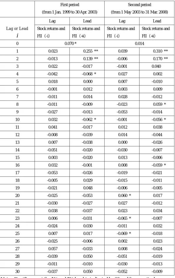
) are insignificant at all cases.4 In the second step of the CCF approach, the standardized residuals and its squares were obtained from the estimates of the conditional means and variances in the first step, and the causality-in-mean and the causality-in-variance are tested based on the sample cross correlation coefficients.

Table 5 shows the test statistic (

T

r

ˆ

_εξ

( )

i

) to test the null hypothesis of no causality-in-mean in the first period and the second period respectively. “Lag” in the table refers to the number of periods stock returns lag FII flows, while “Lead” refers to the number of periods they lead FII flows. The significant test statistics at a specific number of Lag (

i

) implies that the return on

2

Q

3

Hamori(2003) summarized the advantages of the EGARCH model over the standard GARCH model.

4

Table 3 and Table 4 also show the Ljung-Box test statistics (

Q

(20) and (20)) . From this, it was found that the null hypothesis of no autocorrelation up to order 20 is accepted both for standardized residuals and their squares in all cases. Therefore, the diagnostic results

stock influences net FII at that point. Similarly, the significant test statistics at a specific number of Lead (

i

) implies that net FII influences stock returns at that point. From this table, it can be seen that during the first period, FII flows did not affect stock returns, but stock returns affected FII flows at lags 1, 2, 4, and 10. On the other hand, during the second period, FII flows affected stock returns at lags 20, 23, and 25, while stock returns affected FII flows at lags 1, 2, 8, 10, and 16.

Similarly, Table 6 shows the test statistic (

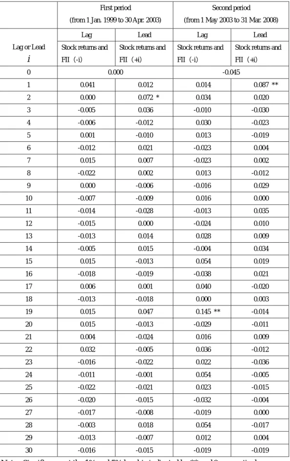
T

r

ˆ

_εξ

( )

i

) to test the null hypothesis of no causality-in- variance in the first period and the second period respectively. As is clear from the table, during the first period, FII flows did not influence stock returns, but stock returns influenced FII flows at lag 2. On the other hand, during the second period, FII flows influenced stock returns at lag 19, while stock returns influenced FII flows at lag 1.

To sum up, this study shows that the return on stock uni-directionally caused FII flows in both mean and variance during the first period, while the return on stock and FII flows were found to induce each other in both mean and variance during the second period. Focusing on the evidence during the second period, it can be seen that FII flows induced stock returns after longer time intervals than stock returns induced FII flows, which is commonly found in the causality-in-mean and the causality-in-variance.

6. Some Concluding Remarks

Since the middle of 2003, the significant increase in the inflow of FII into India has made it the primary source of portfolio investment. Given the dominant role of equity in FII flows and the relative thinness of the Indian capital market, the surge of FII inflows is considered to have affected stock price movements in the country. The stock index has shown a significant upward movement since the middle of 2003. Previous studies were done prior to this upward movement. Moreover, they used daily and/or monthly data from before 2003, and only found an impact from stock returns on FII flows. The research in this paper re-examined the causal relationship between net FII flows and Indian stock returns during the period before 2003, then went on to examine the period since that date. It used daily data from 1 January 1999 to 30 April 2003 to re-examine the first period, and data from 1 May 2003 to 31 March 2008 for its examination of the second period.

The analysis in this study used two empirical techniques: the CCF approach and the LA-VAR based causality test. The results of the CCF approach show that there has been a bi-directional relationship between stock returns and FII flows both in mean and variance during the period beginning in May 2003, while there was a uni-directional causal relationship from stock returns

to FII flows both in mean and variance during the period before May 2003. This indicates that causality from stock returns to FII flows has taken place in both sample periods, whereas the causality from FII flows to stock returns has only been in the latter period. In terms of the causal directions, the LA-VAR based Granger test supports the results of the CCF approach, which indicates the robustness of the empirical results.

Moreover, focusing on the results of the CCF approach during the period after 2003, it can be seen that FII flows have caused stock returns after longer time intervals than stock returns have caused FII flows, which is seen in both the causality-in-mean and the causality-in-variance. This evidence means that stock-price changes quickly affects the behavior of foreign investors, whereas FII flows take more time to affect stock returns, probably because of other macroeconomic variables such as interest rates, asset prices, reserves, money supply, and inflation (RBI 1996 [61]).

In sum, the findings in this paper, especially during the latter period, suggest that net FII inflows have exerted impacts on the movement of Indian stock prices at longer intervals. Over the last five years, net FII inflows have generally trended upward with the movement of stock prices in India. After the peak in mid-January 2008, however, both significantly reversed this trend; FII inflows have turned into persistent outflows, and stock prices have decreased at a record pace. Under these circumstances, given the results in this paper, it can be concluded that when monitor the movement of future stock prices, the authorities will have to pay more attention to FII flows than they have in the past.

References

Bhar, Ramaprasad, and Shigeyuki Hamori. 2008. “Information Content of Commodity Futures Prices for Monetary Policy.” Economic Modelling 25, no. 2: 274-283.

Chakrabarti, Rajesh. 2001. “FII Flows to India: Nature and Causes.” ICRA Bulletin Money and Finance, Oct-Dec: 61-81.

Chandrasekhar, C. P., and Parthapratim Pal. 2006. “Financial Liberalization in India: An Assessment of its Nature and Outcomes.” Economic and Political Weekly 41, no. 11: 975-985.

Cheung, Yin-Wong, and Lilian K. Ng. 1996. “A Causality-in-Variance Test and its Application to Financial Market Prices.” Journal of Econometrics 72, nos. 1-2: 33-48.

Fundamentals Matter?” IMF Working Paper, WP/03/20.

Griffin, John M., Federico Nardari, and Rene M. Stulz. 2002. “Daily Cross-Border Equity Flows: Pushed or Pulled ?” NBER Working Paper Series, no. 9000.

Hamori, Shigeyuki. 2003. An Empirical Investigation of Stock Markets: The CCF Approach, Boston: Kluwer Academic.

Hayashi, Fumio. 2000. Econometrics, Princeton, N.J.: Princeton University Press.

Hong, Yongmiao. 2001. “A Test for Volatility Spillover with Application to Exchange Rate.” Journal of Econometrics 103, nos. 1-2; 183-224.

Mukherjee, Paramita, Suchismita Bose, and Dipankor Coondoo. 2002. “Foreign Institutional Investment in the Indian Equity Market: An Analysis of Daily Flows during January 1999-May 2002.” ICRA Bulletin Money and Finance, April-Sept: 21-51.

Reserve Bank of India. 1996. Annual Report 1995-96, Mumbai: RBI. Reserve Bank of India. 2008a. Annual Report 2007-08, Mumbai:

Reserve Bank of India. 2008b. Handbook of Statistics on Indian Economy 2007-08, Mumbai: RBI.

Toda, Hiro Y., and Taku Yamamoto. 1995. “Statistical Inference in Vector Autoregressions with Possibly Integrated Processes.” Journal of Econometrics 66, nos. 1-2, pp.225-250.

Figure 1: Cumulative Net FII and Stock Price Index 0 50000 100000 150000 200000 250000 300000 Jan-93 Jan-94 Jan-95 Jan-96 Jan-97 Jan-98 Jan-99 Jan-00 Jan-01 Jan-02 Jan-03 Jan-04 Jan-05 Jan-06 Jan-07 Jan-08 F II ( R s. cr o re) 0 5000 10000 15000 20000 25000 Pr ic e I n d e x

Source: Datastream and RBI(2008b).

Note: The bold line is the cumulative net FII and the dotted line is BSE SENSEX 30 stock price index.

Table 1: Causality from LA-VAR (

d

_max= 1) (from 1 January 1999 to 30 April 2003)

Explained variables Explanatory variables Stock returns FII

Stock returns − 18.924

FII 103.884 ** −

(from 1 May 2003 to 31 March 2008)

Explained variables Explanatory variables Stock returns FII

Stock returns − 39.337 **

FII 342.758 ** −

Note 1: Numbers in the table are the Wald test statistics.

Note 2: ** and * indicate that the null hypothesis of Granger non-causality is rejected at the 1% and 5% significance level respectively.

Table 2: Causality from LA-VAR (

d

_max= 2) (from 1 January 1999 to 30 April 2003)

Explained variables Explanatory variables Stock returns FII

Stock returns − 18.568

FII 102.115 ** −

(from 1 May 2003 to 31 March 2008)

Explained variables Explanatory variables Stock returns FII

Stock returns − 42.275 **

FII 336.730 ** −

Note 1: Numbers in the table are the Wald test statistics.

Note 2: ** and * indicate that the null hypothesis of Granger non-causality is rejected at the 1% and 5% significance level respectively.

Table 3: Empirical Results of the AR-EGARCH Model (from 1 January 1999 to 30 April 2003) AR(m)

y

t ＝

π

0 ＋ t i ＋ m i iy− =

∑

1

π

ε

t EGARCH(1,1) log

δ

t2 ＝

ϕ

＋ 1 1 − − t t

δ

ε

α

＋

β

log

( )

δ

t2−1 ＋ 1 1 − − t t

δ

ε

γ

Stock Returns FII

Model AR(9)-EGARCH(1,1) AR(9)-EGARCH(1,1) Estimates Standard Error Estimates Standard Error

AR(m) 0

π

-0.321 1.512 9.268 ** 2.782 1

π

0.048 0.033 0.210 ** 0.043 2

π

0.009 0.038 0.128 ** 0.036 3

π

0.026 0.033 0.048 0.031 4

π

0.078 * 0.031 -0.009 0.038 5

π

-0.024 0.036 0.043 0.034 6

π

-0.070 * 0.034 -0.023 0.038 7

π

0.005 0.032 -0.013 0.044 8

π

0.034 0.034 0.066 * 0.031 9

π

0.075 * 0.032 0.053 0.037 EGARCH(1,1)

ϕ

-0.047 0.049 0.084 0.059

α

0.193 ** 0.051 0.130 ** 0.034

β

0.988 ** 0.006 0.982 ** 0.006

γ

-0.056 0.350 -0.087 0.077 Log Likelihood -5847.192 -6441.295 Q(20)（P-value） 0.230 0.715 2

Q

(20)（P-value） 0.962 0.904

Note 1: Significance at the 1% and 5% level is indicated by ** and *, respectively.

Note 2: Both (20) and (20) are a Ljung-Box test statistic for the null hypothesis that there is no autocorrelation up to order of 20 for standardized residuals and their squares respectively. The number in the figure is the P-value. If this value is less than 0.01 and/or 0.05, the null hypothesis is rejected at the 1 % and 5% level respectively.

Q

Q

2

Note 3: The standard errors are Bollerslev-Wooldrige robust standard errors, which are robust to departures from normality.

Table 4: Empirical Results of the AR-EGARCH Model (from 1 May 2003 to 31 March 2008) AR(m)

y

t ＝

π

0 ＋ t i ＋ m i iy− =

∑

1

π

ε

t EGARCH(1,1) log

δ

t2 ＝

ϕ

＋ 1 1 − − t t

δ

ε

α

＋

β

log

( )

δ

t2−1 ＋ 1 1 − − t t

δ

ε

γ

Stock returns FII

Model AR(10)-EGARCH(1,1) AR(10)-EGARCH(1,1) Estimates Standard Error Estimates Standard Error

AR(m) 0

π

9.447 ** 2.285 32.185 ** 10.917 1

π

0.116 ** 0.031 0.350 ** 0.052 2

π

-0.056 0.032 -0.016 0.066 3

π

0.051 0.034 0.193 ** 0.049 4

π

-0.011 0.029 0.048 0.044 5

π

-0.046 0.033 0.011 0.037 6

π

-0.056 0.031 0.010 0.048 7

π

0.034 0.029 -0.082 0.054 8

π

-0.036 0.029 0.083 * 0.034 9

π

0.030 0.031 0.007 0.038 10

π

0.068 * 0.032 0.103 0.053 EGARCH(1,1)

ϕ

-0.117 * 0.052 0.102 0.122

α

0.307 * 0.047 0.411 ** 0.070

β

0.988 ** 0.005 0.970 ** 0.010

γ

-0.036 0.034 0.005 0.050 Log Likelihood -7513.057 -9149.406 Q(20)（P-value） 0.994 0.294 2

Q

(20)（P-value） 0.843 0.999

Note 1: Significance at the 1% and 5% level is indicated by ** and *, respectively.

Note 2: Both (20) and (20) are a Ljung-Box test statistic for the null hypothesis that there is no autocorrelation up to order of 20 for standardized residuals and their squares respectively. The number in the figure is the P-value. If this value is less than 0.01 and/or 0.05, the null hypothesis is rejected at the 1 % and 5% level respectively.

Q

Q

2

Note 3: The standard errors are Bollerslev-Wooldrige robust standard errors, which are robust to departures from normality.

Table 5: Causality in Mean between FII Flows and Stock Returns

First period

(from 1 Jan. 1999 to 30 Apr. 2003)

Second period

(from 1 May 2003 to 31 Mar. 2008)

Lag or Lead

i

Lag Lead Lag Lead Stock returns and

FII（-i）

Stock returns and FII（+i）

Stock returns and FII（-i）

Stock returns and FII（+i） 0 0.070 * 0.014 1 0.023 0.255 ** 0.039 0.310 ** 2 -0.013 0.139 ** -0.006 0.170 ** 3 0.022 -0.017 -0.001 0.040 4 -0.042 -0.068 * 0.027 0.002 5 0.018 0.000 0.007 -0.010 6 -0.001 0.012 0.003 0.009 7 -0.011 0.014 0.028 -0.012 8 -0.011 -0.009 -0.023 0.059 * 9 -0.027 -0.013 -0.053 -0.014 10 0.032 -0.062 * -0.001 -0.056 * 11 0.041 -0.017 0.012 0.038 12 -0.008 -0.039 0.014 -0.044 13 0.007 -0.038 0.000 -0.026 14 -0.051 -0.020 -0.030 -0.007 15 0.003 -0.020 0.013 -0.006 16 0.032 -0.001 0.008 -0.059 * 17 -0.053 -0.026 -0.019 -0.021 18 -0.005 0.029 -0.015 -0.011 19 -0.021 0.048 -0.006 -0.005 20 -0.025 -0.053 0.060 * 0.017 21 -0.030 -0.027 0.027 -0.012 22 0.038 -0.037 0.023 0.034 23 0.006 -0.031 -0.065 * -0.007 24 -0.024 0.030 -0.011 0.032 25 0.007 0.017 -0.069 * -0.018 26 -0.025 -0.006 0.002 0.023 27 0.057 -0.033 0.008 -0.024 28 -0.039 0.050 -0.051 -0.019 29 -0.011 -0.010 -0.030 -0.013 30 -0.037 0.050 -0.052 -0.009

Table 6: Causality in Variance between FII Flows and Stock Returns

First period

(from 1 Jan. 1999 to 30 Apr. 2003)

Second period

(from 1 May 2003 to 31 Mar. 2008)

Lag or Lead

i

Lag Lead Lag Lead Stock returns and

FII（-i）

Stock returns and FII（+i）

Stock returns and FII（-i）

Stock returns and FII（+i） 0 0.000 -0.045 1 0.041 0.012 0.014 0.087 ** 2 0.000 0.072 * 0.034 0.020 3 -0.005 0.036 -0.010 -0.030 4 -0.006 -0.012 0.030 -0.023 5 0.001 -0.010 0.013 -0.019 6 -0.012 0.021 -0.023 0.004 7 0.015 0.007 -0.023 0.002 8 -0.022 0.002 0.013 -0.012 9 0.000 -0.006 -0.016 0.029 10 -0.007 -0.009 0.016 0.000 11 -0.014 -0.028 -0.013 0.035 12 -0.015 0.000 -0.024 0.010 13 -0.013 0.014 0.028 0.009 14 -0.005 0.015 -0.004 0.034 15 0.015 -0.013 0.054 0.019 16 -0.018 -0.019 -0.038 0.021 17 0.006 0.001 0.040 -0.020 18 -0.013 -0.018 0.000 0.003 19 0.015 0.047 0.145 ** -0.014 20 0.015 -0.013 -0.029 -0.011 21 0.004 -0.024 0.016 0.009 22 0.032 -0.005 0.036 -0.012 23 -0.016 -0.022 0.022 -0.036 24 -0.011 -0.001 0.054 -0.005 25 -0.022 -0.021 0.023 -0.015 26 -0.020 -0.015 -0.032 -0.004 27 -0.017 -0.008 -0.019 0.000 28 -0.003 0.018 0.054 -0.017 29 -0.013 -0.007 0.012 0.004 30 -0.016 -0.015 -0.019 -0.019