第 巻 第 号 抜 刷
年 月 発 行
Monetary policy inertia, macroprudential policy,
and financial stability in a liquidity trap
and financial stability in a liquidity trap
*Kohei Hasui
†abstract
After the colossal financial crisis of , many monetary policy analyses have shown the profound implications for financial stability of monetary policy in a liquidity trap. This paper investigates how monetary policy in a liquidity trap affects financial stability in a New Keynesian model incorporating a financial friction. The main findings are as follows : A strong financial stabilization policy is effective in mitigating an excess expansion of credit in normal times. However, this same stabilization policy expands credit when the economy is in a liquidity trap. These findings show that the effectiveness of financial stabilization policy can vary depending on whether or not the economy is in a liquidity trap. JEL Classification : E , E
Keywords : Zero interest rate policy, Financial stability, Credit expansion, Macro-prudential policy
Introduction
After the financial crisis, unconventional monetary policy, such as zero-interest-rate policy, and quantitative and qualitative easing have been conducted in developed countries. Many papers have pointed out that these policy tools have profound implications for stabilizing the economy in a liquidity trap(Eggertsson and Woodford, ; Adam and Billi, ; Gertler and Karadi, ).
Simultane-*This work was supported by JSPS KAKENHI Grant Number JP K . †Associate Professor, Faculty of Economics, Matsuyama University.
ously, the potential importance of financial stabilization, in particular, macropruden-tial policy in terms of system and effectiveness, has been discussed extensively since the financial crisis(Borio, ; Drehmann et al., ; Jeanne, ; Bianchi and Mendoza, ).
In this paper, we investigate simply whether the effectiveness of financial stabilization policy changes when an economy is in a liquidity trap. We introduce the zero lower bound(ZLB)on the nominal interest rate into Suh’s( )model incorporating financial friction a la Iacoviello( )and macroprudential policy. The potential importance of Suh’s( ) model is that monetary policy and macroprudential policy is structured separately in the model framework. This enables us to analyze the effectiveness of financial stabilization, distinguishing macroprudential policy from monetary policy. In Suh’s( )model, the finan-cial intermediary faces several costs : First, borrowers receive windfall income when a loan is bad. This windfall income is financed by the financial intermediary’s cost, which assumes increasing function of the loan. Second, the financial intermediary faces the regulation of credit expansion. Financial intermediaries have to pay the penalty cost if they violate the regulation. Finally, the financial intermediary has to pay interest for a loan. The financial intermediary maximizes the profit subject to these costs(constraints). Due to this framework, policy rate and credit expansion depend on both macroprudential policy and monetary policy.
We find that strong financial stabilization policy is effective in mitigating an excess expansion of credit in normal times. However, this same strong stabilization policy expands credit when the economy is in a liquidity trap. In our analysis, higher financial regulation applies downward pressure on the nominal interest rate. This makes the zero-interest rate policy longer, and financial stability worsens. These findings show that the effectiveness of financial stabilization policy can vary depending on whether or not the economy is in a liquidity trap.
Recently, some papers introduce the ZLB into the model a la Iacoviello ( ): Rubio and Yao( )analyze the effectiveness of macroprudential policy by defining macro-prudential policy as regulating the excess expansion of credit. They show that monetary policy and macroprudential policy can perfectly coordinate in stabilizing the economy in normal times, but this effectiveness of coordination does not hold straightforwardly when the economy is in a liquidity trap. Unlike Suh’s( )analysis, Rubio and Yao( )analyze the financial stabilization in a unified framework of macroprudential policy and monetary policy. Our paper complements the work of Rubio and Yao( )and Suh( )in terms of the liquidity trap, as well as distinguishing between monetary policy and macropruden-tial policy to show that strong financial stabilization policy can expand credit when the economy is in a liquidity trap).
Recently, some studies have analyzed the effectiveness of macroprudential policy in a liquidity trap : Antipa and Matheron( )and Wu and Zhang( ) show that a macroprudential policy can complement the forward-guidance in the liquidity trap. Lewis and Villa( ) demonstrate that capital regulation is effective in a liquidity trap. Korinek and Simsek( )find that by limiting debts, macroprudential policy can improve social welfare in a liquidity trap.
The remainder of this paper is as follows. Section describes the model. In Section , we explain the results by deriving impulse responses. Section concludes the paper.
)In analyses of the macroprudential policy, the borrowing and liquidity constraints are introduced into households and banking sectors frequently : Farhi and Werning( )analyze the macroprudential policy by introducing the borrowing constraint into the model with nominal regidities in goods market and labor market. Gertler and Kiyotaki( )analyze performance of the macroprudential policy by introducing the borrowing and liquidity constraint into the banking sector.
The model
The model is Suh( ), incorporating financial friction a la Iacoviello ( )) ! ! &+",# ,&+","!! ! *&$(,! ,),"!%"!*&-'"," ( ) ! ! &%",# ,&%","!!! *&$*%",! ,),"!%" !*&-'"," ( ) ! ),#$ ,),"!"($'+&+","'%&%",!$!"*"%$,%" ( ) ! #,,! ! $%#$*%",!!!),",,!!%#%%&%","%+&+","%$$," ( ) *%",#(,"$+"&,%,," ( ) where
'+#)+*&"&+*)"'%#)%*&"&%*)"
%+#!."% # $!"!#*)%'+"%%#&%"%+"."% *) ."% # " %$#!."% # $!"*)%!
&+",, &%",, ),, (,, *%",, and,,denote consumption of saving households, consumption of borrowers, inflation rate, nominal interest rate, borrowing rate, and debt of borrowers(i. e., deposit of saving households), respectively. Parameters $, $%,
*&, and *)denote the subjective discount factor of saving households, subjective discount factor of borrowers, relative risk aversion of saving households, relative risk aversion of borrowers, and preference for labor supply, respectively. + denotes degree of cost of financing the windfall income, and &,denotes degree of
)We describe the log-linearized model around the steady state. See appendix of the present paper or Suh( )for detailed derivation of the model.
response to debt in macroprudential policy. A higher#&means that
macropruden-tial regulation is tighter. !"# denotes debt-output ratio at the steady state ; + denotes the real wage at the steady state ; and "%"# denotes borrower’s labor
supply-output ratio at the steady state.
Equations( )and( )denote the Euler equation of saving households and borrowers, re-spectively. These equations are derived from saving households’ and borrowers’ intertemporal consumption decisions. Equation( )denotes the Phillips curve, which is derived from the firm’s optimal price setting.
Equations( )and( )are derived from the financial intermediary’s optimal decision. As in Curdia and Woodford’s( )model, the financial intermediary intermediates between saving households and borrowers, but this intermediation has costs. Moreover, the financial intermediary cannot predict which loan will go bad, but can know the fraction of bad loans to all loans. In Suh’s( )model, cost is an increasing function of intermediation. Moreover, the financial intermediary faces the regulation of macroprudential policy. Financial intermediaries must pay the cost if they violate the regulation of credit expansion. Therefore, the financial intermediary must maximize profits facing these two types of costs. Due to these factors, the nominal interest rate(policy rate) and borrowing rate depend on monetary policy and macroprudential policy. Finally, we note that . t is treated as the credit expansion, i. e., degree of financial stability. A low credit expansion means higher financial stability.
Monetary policy is given by following interest rate rule with ZLB.
')$#"$'!(#!%'')!!"%!!%'&%#$$)"#'')&(! ( )
where(#denotes the real interest rate at the steady state, and%'denotes the inertia of the policy rate.
Finally, *&!)and$)denote demand shock and productivity shock, respectively.
These variables follow an exogenous process as follows :
'$"&#'$'$"&!""*&$" ( )
!&#'!!&!""*&!" ( )
'$ and '! denote persistence of demand shock and productivity shock, respec-tively. *&$and*&!are the i. i. d disturbance term.
Results
Parameters Values Explanation
# . Subjective discount factor(saving households)
#" . Subjective discount factor(borrowers)
(# Intertemporal substitution of consumption
(% Preference for labor supply
) . Degree of cost of paying windfall income
% . Elasticity of inflation to real marginal cost
$& . Response to inflation rate in policy rule
$, Response to output in policy rule
$+ . Response to credit spread in macroprudential policy
'$ . Persistence of demand shock
'! . Persistence of productivity shock
Std . Standard deviation of the shocks
Table : Parameter Values
In this section, we derive the impulse responses to a negative demand shock.) Table indicates calibration. Following Suh( ), we set parameter
values as follows : ##!!((##, #"#!!('($, (##", (%#", )#!!!#, %#!!"&.
For policy parameters, we set $&#"!%, $,#!, and $+#!!".) We set '$#
)See Miranda and Fackler( )for deriving impulse response with the ZLB. )Suh( )sets$+#!!"%.
6 4 2 0 8 10 12 14 16 18 20 6 4 2 0 8 10 12 14 16 18 20 6 4 2 0 8 10 12 14 16 18 20 -30 -20 -10 0 10 0 10 20 -3 -2 -1 0
"!!!!%, and set the standard deviation of the shock as !!". Debt-output ratio at
the steady state, the fraction of borrowers’ labor supply to aggregate labor supply, consumption-output ratio, and output-aggregate labor supply ratio are set !!'&', !!%#, !!$', and ", respectively.
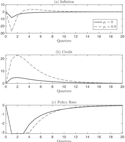
First, we analyze how financial stability changes by deriving the impulse response to negative demand shock. Figure shows the impulse responses to
Figure : Impulse response to − % annual shock of ud,t
6 4 2 0 8 10 12 14 16 18 20 6 4 2 0 8 10 12 14 16 18 20 6 4 2 0 8 10 12 14 16 18 20 -40 -20 0 20 0 10 20 -6 -4 -2 0
− % annual shock of$!"#under#"!!and #"!!!". According to the figure, the
nominal interest rate(policy rate)takes off from the ZLB smaller in the case of #"!!!"than the case of #"!!. As previous studies have shown, such longer
zero interest rate policy is effective in the liquidity trap(Eggertsson and Woodford, ; Jung et al., ; Adam and Billi, ; Nakov, ).
However, financial stability worsens when #"!!!"(Panel (b)). This is
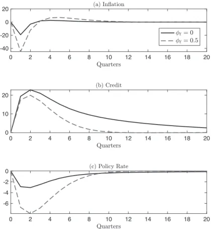
Figure : Impulse response to − % annual shock of ud,t under !"= and !"= .(without a ZLB)
6 4 2 0 8 10 12 14 16 18 20 6 4 2 0 8 10 12 14 16 18 20 6 4 2 0 8 10 12 14 16 18 20 -100 -50 0 0 20 40 -3 -2 -1 0
because the delayed lift off from the ZLB decreases borrowing costs. Simultane-ously, the economic agent expects the zero-interest rate policy will continue longer due to the higher policy inertia and this amplifies the effect. Therefore, although policy tools such as forward-guidance are effective in the liquidity trap to stabilize the economic recession, they can worsen financial stability.
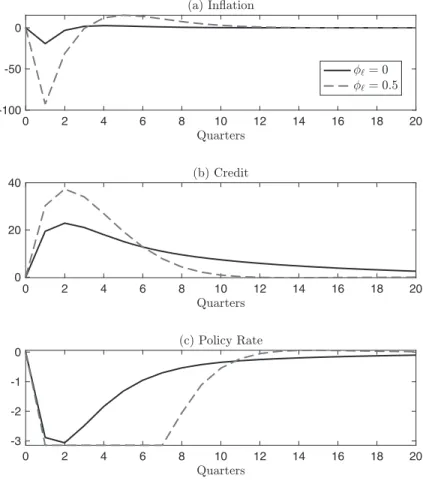
Figure : Impulse response to − % annual shock of ud,t under !"= and !"= .(with the ZLB)
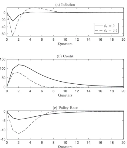
Next we analyze how degree of financial regulation #% affects financial
stability. Figure shows the impulse responses to− % annual shock of$!"#under #%!!and #%!!!", where we do not impose a ZLB.) As may be seen in the
figure, the credit response becomes smaller in the case of#%!!!"than of #%!!.
The financial stability improves as #%increases. This result shows that financial
regulation is effective in stabilizing credit expansion. On the other hand, the nominal interest rate decreases more when #%!!!" than when #%!!. As
explained in the previous section, the nominal interest rate and credit are affected by macroprudential policy. An increase in #%applies a downward pressure on the
nominal interest rate, as shown by Eq.( ).
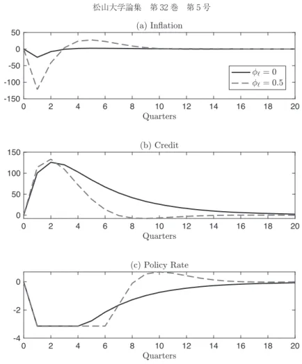
Next we show that this result changes when we consider the effect of the ZLB on the nominal interest rate. Figure shows that the impulse responses to − % annual shock of $!"#under #%!!and #%!!!", where we impose the ZLB on the
nominal interest rate. According to the figure, the credit response is larger when #%!!!"than when #%!!. Moreover, zero-interest rate policy continues quite a
bit longer in the case of#%!!!"than the case of #%!!. Combining the result of
Figure , an increase in #%applies the downward pressure on the nominal interest
rate. This makes the zero interest rate policy last longer, and hence financial stability worsens. Therefore, the effectiveness of macroprudential policy for stabilizing credit expansion can change when the economy is in a liquidity trap.)
Conclusion
This paper investigated how monetary policy in a liquidity trap affects financial stability in a New Keynesian model incorporating a financial friction. We obtained
)We set$"!!!#.
)In appendix of the paper, we show that the result of Figure changes under alternative parameter values.
findings as follows : A strong financial stabilization policy is effective in mitigating a excess expansion of credit in a normal time. However, this strong stabilization policy also expanded credit when the economy was in a liquidity trap. This shows that the effectiveness of the financial stabilization policy could be altered depending on whether or not the economy is in a liquidity trap.
However, we simplify the introduction of financial friction and macroprudential policy. Therefore, we did not consider the role of the net worth of the firm sector or financial sector(Bernanke et al., ; Gertler and Karadi, ). Moreover, we imposed the ZLB on the policy rate only, not on the borrowing rate. Therefore, we could not capture the effect of binding the ZLB in the borrowing rate. More detailed analysis is needed on these issues.
Finally, we do not explain the intuition why higher financial regulation decreases the policy rate more. It is difficult to consider that this mechanism is robust. Therefore, we need further analysis on the relation between macropruden-tial policy and the policy rate.
Appendix
A. Brief description of Suh( )
In this section, we present a brief overview of the Suh’s( )model. First, household sector consists of saving households and borrowers. The saving households are patient(i. e., higher subjective discount factor), and the borrowers impatient(i. e., lower subjective discount factor).
The problem of saving households is given as follows :
$#% !'!(!#'!(" !# (#! $ "(% (% !'!( "!#$ "!#$!$ #'!""#( & ""#& ! "! s. t. (A. )
"/"0"%/"0
'0#(0!"
%/"0!"
'0 "10&/"0"#/"0"
Analogously, the problem of borrowers is given as follows. %#& "*"0"&*"0$ !# 0#! $ #*0)0, "*"0 "!&+ "!&+!( &*"""&0. ""&. ! "" s. t. (A. ) "*"0"(*"0!"%*"0!" '0 #% *"0 '0"10&*"0"#/"0"
where, "/"0, "*"0, %/"0, %*"0, &/"0, &*"0, and 10denote consumption of saving house-holds, consumption of borrowers, deposit of saving househouse-holds, debt of borrowers, labor supply of saving households, and labor supply of borrowers, respec-tively. #/"0 denotes saving households’ profit from the intermediate goods sector. #*"0denotes the borrowers’ windfall income when the borrowing is bad.
Intermediate goods firm - produces )-"0#!0&-"0 facing the monopolistic
competition. The final goods firm aggregates these goods. Optimal price-setting is analogous to the standard New Keynesian model. Hence, we obtain the following Phillips curve.
!
%0## 0%0"""$%$0" (A. )
where %$0denotes the real marginal costs. Finally, we describe the financial intermediary. The financial intermediary maximizes the profit as follows :
%#&
*0 (
*"0*0!'%*0&! (A. )
where '%*0&denotes the cost. The financial intermediary faces several costs :
First, the borrowers receive a windfall income when a loan is bad. This windfall income is financed by the financial intermediary’s cost Ω. It is assumed that the
cost Ω is an increasing function of the loan +'. Second, the financial intermediary faces the regulation of credit expansion. The financial intermediary has to pay the penalty cost Ξtif they violates the regulation. Analogous to Ω, we assume that Ξt
is an increasing function of +'. Finally, the financial intermediary has to pay interest !' on one unit of loan +'. Combining these costs, the financial intermediary maximizes the profit(A. )subject to the following constraints :
Ω Ξ
*$+'%#!'+'" $+'%" $+'%"
Ω$+'%#Ω!+'("
Ξ$+'%#Ξ!+'$+!
Therefore, we treat $+as the degree of financial stabilization policy. Solving this problem yields the following relation :
Ω
!""'#$"!(!$+% )!&"'+'"!(!$+! (A. )
Equation(A. ) shows that parameters of macroprudential policy affects the borrowing rate!""'.
A. Robustness
The case for $!!""&!#%and #!!!!#$
In this section, we derive the impulse responses to a negative demand shock under alternative parameter values. We set '##"#&!#%and %#!!!#$following
Rotemberg and Woodford( )and Woodford( ).
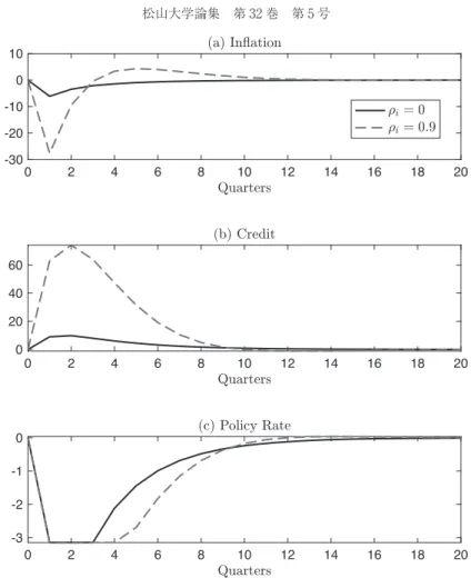
First, we analyze how financial stability changes by deriving the impulse response to the negative demand shock. Figure A shows the impulse responses to − % annual shock of ($"'under '##"#&!#%, %#!!!#$, &%#!, and &%#!!'.
The result does not change from Figure . The nominal interest rate(policy rate)
6 4 2 0 8 10 12 14 16 18 20 6 4 2 0 8 10 12 14 16 18 20 6 4 2 0 8 10 12 14 16 18 20 -30 -20 -10 0 10 0 20 40 60 -3 -2 -1 0
takes off from the ZLB smaller in the case of""!!!"than of $!#"!!.
Analogous to Figure , the financial stability worsens when""!!!". This is
because the delayed lift off from the ZLB decreases the borrowing costs. The economic agent expects that the zero interest rate policy will continue longer due to the higher policy inertia. Therefore, policy tools such as forward-guidance can
Figure A : Impulse response to − % annual shock of%#!$(""= / . ,!= . )
6 4 2 0 8 10 12 14 16 18 20 6 4 2 0 8 10 12 14 16 18 20 6 4 2 0 8 10 12 14 16 18 20 -60 -40 -20 0 0 50 100 150 -15 -10 -5 0
worsen the financial stability.
Next we also analyze how degree of financial regulation#$affects the financial
stability. Figure A shows the impulse responses to − % annual shock of #!""
under #$!!and #$!!!", where we do not impose the ZLB.)Analogous to
Figure , the response of the credit becomes smaller under the case of#$!!!"than Figure A : Impulse response to − % annual shock of%#!$under#"= / . ,
"= . , !$= , and!$= .(without the ZLB) and financial stability in a liquidity trap
6 4 2 0 8 10 12 14 16 18 20 6 4 2 0 8 10 12 14 16 18 20 6 4 2 0 8 10 12 14 16 18 20 -150 -100 -50 0 50 0 50 100 150 -4 -2 0
under the case of !"!!. The financial stability improves as !"increases. This result shows that the financial regulation is effective to stabilize the credit expansion under alternative parameter values. Moreover, the nominal interest rate decreases
)We set the value of the shock − % so that the nominal interest rate binds the ZLB. Figure A : Impulse response to − % annual shock of%#!$under#"= / . ,
more under the case of $(!!!%than under the case of $(!!. This is also same
as Figure .
Next we show that this result changes when we consider the ZLB on the nominal interest rate. Figure A shows that the impulse responses to − % annual shock of $""#under '!!"#&!#%, %!!!!#$, $(!!, and $(!!!%, where we
impose the ZLB on the nominal interest rate. The result changed from the result of Figure . According to the figure, credit responds slightly larger until second quarter, but decrease more after second quarter in the case of$(!!!%than the case
of $(!!. Moreover, the zero interest rate policy continues longer in the case of
$(!!!%than in the case of $(!!, but the nominal interest rate policy increases
faster in the case of $(!!!%than of $(!!. This large overshoot tightens the
credit expansion. Therefore, the effectiveness of stronger financial stabilization policy is improved in the liquidity trap under '!!"#&!#% and %!!!!#$.
Combining the result of Figure A , whether the effectiveness of the macroprudential policy depends parameter values other than policy parameters.
The case for !"!!
Finally, we set policy parameter alternative value. We set $&!%, which the
interest rate responds higher to the inflation rate. Figure A shows that the impulse responses to − % annual shock of $""#under $&!%, '!!"#&!#%, %!!!!#$,
$(!!, and $(!!!%, where we impose the ZLB on the nominal interest rate. The
result did not change from the result of Figure A . According to the figure, credit responds slightly larger until second quarter, but decrease more after second quarter in the case of $(!!!%than of $(!!. Moreover, the zero interest rate policy
continues longer under the case of $(!!!%than in the case of $(!!, but the
nominal interest rate policy increases faster in the case of$(!!!%of $(!!.
6 4 2 0 8 10 12 14 16 18 6 4 2 0 8 10 12 14 16 18 20 20 6 4 2 0 8 10 12 14 16 18 20 -150 -100 -50 0 50 0 50 100 150 -4 -2 0 2 References
Adam, K. and R. M. Billi( )“Optimal monetary policy under commitment with a zero bound on nominal interest rates,”Journal of Money, Credit and Banking , − .
Antipa, P. and J. Matheron( )“Interactions between monetary and macroprudential policies,” Financial Stability Review − .
Bernanke, B. S., M. Gertler, and S. Gilchrist( )“The financial accelerator in a quantitative Figure A : Impulse response to − % annual shock of%#!$under#"= / . ,
business cycle framework,”in Handbook of Macroeconomics, ed. by J. Taylor and M. Woodford Elsevier vol. chap. , − .
Bianchi, J. and E. G. Mendoza( )“Optimal Time-consistent macroprudential policy,”Journal of Political Economy , − .
Borio, C.( )“Rediscovering the macroeconomic roots of financial stability policy : journey, challenges and a way forward,”BIS Working Papers Bank for International Settlements. Curdia, V. and M. Woodford( )“Credit spreads and monetary policy,”Journal of Money,
Credit and Banking , − .
Drehmann, M., C. Borio, and K. Tsatsaronis( )“Characterising the financial cycle : don’t lose sight of the medium term !” BIS Working Papers Bank for International Settlements. Eggertsson, G. B. and M. Woodford( )“Zero bound on interest rates and optimal monetary
policy,”Brookings Papers on Economic Activity , − .
Farhi, E. and I. Werning( )“A theory of macroprudential policies in the presence of nom-inal rigidities,”Econometrica , − .
Gertler, M. and P. Karadi( )“A model of unconventional monetary policy,”Journal of Monetary Economics , − .
Gertler, M. and N. Kiyotaki( )“Financial Intermediation and credit policy in business cycle analysis,” in Handbook of Monetary Economics, ed. by B. M. Friedman and M. Woodford Elsevier vol. of Handbook of Monetary Economics chap. , − .
Iacoviello, M.( )“House prices, borrowing constraints, and monetary policy in the business cycle,”American Economic Review , − .
Jeanne, O.( )“The macroprudential role of international reserves,” American Economic Review , − .
Jung, T., Y. Teranishi, and T. Watanabe( )“Optimal monetary policy at the zero-interest-rate bound,”Journal of Money, Credit, and Banking , − .
Korinek, A. and A. Simsek( )“Liquidity trap and excessive leverage,”American Economic Review , − .
Lewis, V. and S. Villa( )“The interdependence of monetary and macroprudential policy under the zero lower bound,”Working Paper Research National Bank of Belgium.
Miranda, M. J. and P. L. Fackler( ) Applied computational economics and finance MIT press.
Nakov, A.( )“Optimal and simple monetary policy rules with zero floor on the nominal interest rate,”International Journal of Central Banking , − .
Rotemberg, J. and M. Woodford( )“An optimization-based econometric framework for the evaluation of monetary policy,”in NBER Macroeconomics Annual , Volume National Bureau of Economic Research, Inc NBER Chapters − .
Rubio, M. and F. Yao( )“Macroprudential policies in a low interest rate environment,” Journal of Money, Credit and Banking , − .
Suh, H.( )“Dichotomy between macroprudential policy and monetary policy on credit and inflation,”Economics Letters , − .
Woodford, M.( ) Interest and Prices : Foundation of a theory of monetary policy Princeton University Press.
Wu, J. C. and J. Zhang( )“A shadow rate New Keynesian model,”Journal of Economic Dynamics and Control , − .