Vol. 61, No. 2, April 2018, pp. 217–235
DYNAMIC INVENTORY CONTROL MODEL WITH FLEXIBLE SUPPLY NETWORK
Kimitoshi Sato Naoya Takezawa
Kanagawa University Nanzan University
(Received April 28, 2017; Revised September 6, 2017)
Abstract In this paper, we consider the inventory problem of a firm facing disruption probability in its supply chain which consists of multiple suppliers and multiple demand nodes. The firm wishes to minimize its total expected cost in a finite time horizon setting. In order to manage the supply chain disruption, we introduce flexibility into the supply chain network of our inventory management problem. The problem is formulated as a Markov decision process, and a state-dependent optimal threshold policy is derived. We show that the expected cost function is monotonic in the convex ordering of the demand distribution and that the optimal policy can be characterized with the ratio of the ordering cost and the disruption probability of supply. We also numerically demonstrate that the flexibility of the supply chain network reduces the total expected cost.
Keywords: Inventory, Disruption probability, Supply chain network, Markov-modulated demand, Dynamic Programming
1. Introduction
The management of supply chain disruption has drawn attention as firms have become more interested in diversifying their production facilities via outsourcing. Such work has been reviewed in Tang [14] and Synder [13]. This paper focuses on the disruption in the supply chain, and models this disruption by considering a state dependent supply network and a state dependent demand distribution whose state follows a Markov chain. The importance of properly managing such disruptions as well as the various sources that potentially affect the supply chain has been discussed in Tang [15]. Among the various sources, we focus on the disruptions that occur due to “complete failure of transportation from a facility” and/or “complete loss of production of a facility”. There are many ways to deal with such a disruption, and we attempt to create resilience in the supply chain by considering flexibility in the transportation network of products rather than altering the production capacity, supply and/or demand of final goods∗.
The proper management of transportation failure risks when the demand distribution is stochastic, does not only prevent disruptions in the downstream of the supply chain, but may also increase the overall efficiency of production at the firm level as well as the industry level. In short, this paper attempts to manage the supply chain disruption probability by introducing flexibility in the supply transportation network instead of optimizing production capacity, etc., when there is a disruption in the delivery process of products. Because we only consider a complete shutdown from a particular facility, the theoretical treatment of failure in the transportation and production become indistinguishable in our case.
∗In such a situation, the yield uncertainty does not become a major issue and will not be considered in this paper.
The practical importance of managing transportation disruption probability in the sup-ply chain, has drawn increasing attention in Japan, especially after the 2011 East Japan Earthquake. Many domestic corporations have become aware of the importance and have become interested in diversifying their production facilities in order to accommodate the product supply via constructing a flexible supply network and/or allocating multiple poten-tial suppliers. In the inventory management literature, the supply chain disruption proba-bility may be categorized as a partial disruption probaproba-bility defined as the lack of supply due to human error or product defects. However, the disruption probability considered in this paper is defined as the complete loss of delivery of products due to loss of transportation infrastructure and/or strike.
2. Literature Review
Many papers have analyzed the supply chain and its disruption probability. Mieghem [16] deals with the production risk by altering the demand via adjusting the price of final goods to be delivered. Jordan and Graves [6] discuss about the process flexibility and how to add production capacity when facing potential production failure. When potential failure may be correlated, Sak and Haks¨oz [11] deal with this phenomenon by using delivery contracts, but we do not use such contracts to mitigate risk†. The proposed model in this paper differs from these paper in the sense that it dose not try to achieve the total cost minimization by either altering the supply production capacity and/or adjusting the price so that the demand meets the supply. The risk originating from the disruption is mitigated by rerouting the excess supply production capacity created by the transportation disruption. Thus, there is no incentive to share or hedge such risk using some kind of supply contract‡.
Tang [15] provides a list of various risks that may affect the supply chain, and among these risks, this paper is most related to the transportation disruption. The paper con-tributes to the literature in the sense that it fills in the gap of supply chain disruption probability by focusing on the transportation flexibility and/or complete loss of production at a particular facility. The originality lies in the way we model the transportation network, which is considered to depend on a state variable that follows a Markov process with a finite time horizon. This allows us to analyze the transient policy instead of the steady state pol-icy, which is more valuable in practice. In addition, the model does not consider production capacity that is dedicated to fulfill the demand shortfall (backup capacity). Instead, we may use any production facility to serve as a backup supplier, which may be useful in practical applications. By using transportation flexibility to deal with such supply chain disruptions, we derive an easy to implement risk adjusted cost index that allows us to construct a pol-icy that introduces flexibility in a supply chain facing disruption probability. This index shares some features with the GBE index proposed in Saghafian and van Oyen [10]. The the cost and disruption probability term become the same when (i) the demand at each point are the same, (ii) a single backup supplier only supplies products to demand points. In other words, there are no the main suppliers. (iii) there is no limitation of backup capacity. Unlike Saghafian and van Oyen [10], the production capacity is not filled in by a backup supplier, but rather satisfied by reallocating the excess capacity generated by the failure in the transportation network. Thus, the policy can be easily implemented by altering the
†If the failure of several transportation arcs are correlated, it is theoretically possible to deal with such models in our proposed framework by orthogonalizing (create uncorrelated supply nodes) the supply node arcs.
‡If such a contract exists, this risk does not need to be dealt with and the hedged capacity may be simply removed from the original network in our model.
transportation network. In addition, because the transportation network itself is assumed to be state dependent, the policy can be solved in a dynamic setting (transient state), in comparison to the steady state behavior derived in Saghafian and van Oyen [10]. The model also provides a solution (threshold policy) on how to introduce transportation flexibility in the supply chain network rather than attempting to fill in the shortfall of demand through backup production capacity (or altering the final demand to match the insufficient supply). Gallego and Hu [2] focus on the case when there are partial disruptions in supply, and the demand follows a distribution that depends on a finite time horizon Markov chain. They derive an optimal order policy in a multiple period inventory model exposed to Markov modulated demand/supply with finite capacity. Schmitt and Snyder [12] consider the case when there is a partial and complete disruption in the supply chain, and consider the impact of adding a backup supplier to increase the flexibility in the supply chain. This paper studies the case when there are multiple suppliers and one firm that needs multiple products when there are only complete disruptions in supply. We also consider a backup supplier and analyze whether to supply from this backup supplier or not as well as the quantity of the inventory to be ordered. This model enables us not only to deal with the backup supplier but also consider a complete disruption in the supply chain by setting up multiple supply routes, which differs from Gallego and Hu [2] and Schmitt and Snyder [12].
In comparison, we consider potential backup suppliers (main suppliers) and analyze whether to supply from these backup suppliers or not, and derive the optimal quantity to be ordered. The proposed model enables us not only to deal with potential backup suppliers but also consider complete disruptions in the supply chain. Such disruption is dealt by setting up multiple supply routes.
We consider a supply chain constituting two stages with multiple supply nodes and multiple demand nodes, this allows us to formulate the probabilistic inventory model as a Markov decision process. In this model, we consider the case where the demand distribution is affected by exogenous factors such as weather hazards and/or business conditions. In the following, we derive an optimal policy under each risk factor that minimizes the total cost in a multi-period framework.
The originality of the paper lies in the way we model the supply chain disruption. The disruption is considered to occur in the delivery process which is dealt with creating a flexible procurement network. Thus, the decision is to choose the optimal supply chain network given the failure (total disruption) in the network. The uncertainty is in the demand of the product which is shown to be monotone in the stochastic order of demand. This implies a unique switching threshold policy that can be easily implemented according to the state of the network when the demand uncertainty increases.
The paper is structured as the following. Section 3 introduces the notation and defini-tions. Section 4 and 5 explain the single and multiperiod version of the model, followed by the conclusion in Section 6.
3. Notation and Definitions
The time horizon of the problem is set to be T where each time period t satisfies t ∈
[1,· · · , T ]. There are K supply nodes which deliver L goods to the demand nodes via the
supply chain network. The demand process of each node and the supply chain network can be formulated as a finite Markov chain X(t), t ≥ 0. The state space of the Markov chain has N states such that the state space S can be defined as S ={1, 2, · · · N}.
1 2 3 1 2 Supplier Customer
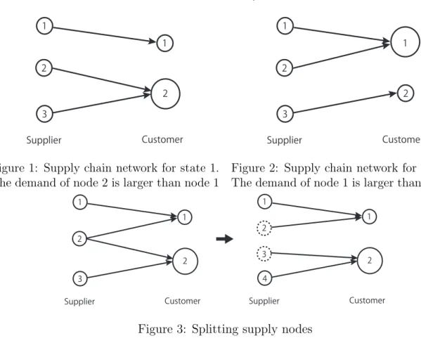
Figure 1: Supply chain network for state 1. The demand of node 2 is larger than node 1
1 2 3 1 2 Supplier Customer
Figure 2: Supply chain network for state 2. The demand of node 1 is larger than node 2
1 2 3 1 2 Supplier Customer 1 2 3 1 2 Supplier Customer 4
Figure 3: Splitting supply nodes
which further allows us to analyze the problem as a Markov decision problem§.
Given the supply chain network structure, we assume the following decision structure at each time period.
1. The state X(t) = i is observed at the beginning of each time period.
2. The quantity of goods from each supply node to each demand node is determined by the supply chain network at state i and the demand node distribution. We assume that there is no lead time in production¶.
3. At the end of each time period, the demand quantity is determined and the inventory is consumed accordingly, and the unsatisfied demand is backlogged.
In the following, we illustrate the notation using an example in Figure 1 and Figure 2 which depicts the case for K = 3 and L = 2. The state i = 1 corresponds to the case when the demand at node 2 is expected to be larger than node 1. In this situation, goods are shipped to demand node 2 from supply node 2 and 3. However, if the state is i = 2, then the demand for node 1 is fulfilled by supply node 1 and 2.
The demand at demand node l in state i is a non-negative random variable Dl(i) with
a cumulative distribution function Fi,l(·). The supply chain network matrix in state i is
defined as C(i) ∈ RK×L where Pij(t) is the transition probability from state i to j with
i, j ∈ S. The element of C(i) is Ckl(i), which satisfies Ckl(i) = 1 if goods are shipped from
supply node k to demand node l, and Ckl(i) = 0 otherwise, i = 1,· · · , N, k = 1, · · · , K,
§Even though the computational complexity of the problem may increase rapidly as the number of de-mand/supply nodes and states of the network increases, it is possible to reduce the computational burden by applying approximations proposed in Federgruen and Zipkin [1], Kunnumkai and Topaloglu [7], [8]. ¶We follow the assumptions in Saghafian and van Oyen [10], which argues that supply lead times and production cycles are negligible in comparison with the review period.
l = 1,· · · , L. Let Cl(i) be the lth vector of supply chain matrix C(i). The supply chain
network matrix C(i) for Figure 1 and Figure 2 become the following.
C(1) = 1 00 1 0 1 , C(2) = 1 01 0 0 1
In our model, we make two assumptions on the demand and the supply nodes. (i) There are at most two suppliers (main supplier and backup supplier) for each demand node, but each supply node can ship goods to multiple demand nodes. (ii) There is no upper limit on the production capacity. This assumption enables us to alter the supply chain network
Ckl(i) by splitting the supply node so that each supply node only ships goods to one demand
node when the supply nodes need to ship goods to multiple demand nodes, i.e. node 2 in Figure 3 is splitted. The two conditions are satisfied if the following Assumption 3.1 holds.
Assumption 3.1. For all k = 1,· · · , Ki and i = 1,· · · , N,
(i) C′k(i)1≤ 2.
(ii) ∑Ll=1Ckl(i)≤ 1.
Ki(≥ K) represents the total number of supply nodes at state i after rearranging the
network so it satisfies Assumption 3.1, and C(i) ∈ RKi×L is the connection matrix of the
network. The value of random variable Rk describes whether supply node k can be
poten-tially supplied or not. If Rk = 1, the node can be supplied and Rk is set to 0 otherwise.
Then, Rk, k = 1, ..., K becomes an i.i.d. Bernoulli random variable, where qk is the
proba-bility of reliaproba-bility.Thus, P (Rk = 1) = qk and P (Rk = 0) = 1− qk hold. Rk and Dl(i) are
assumed to be independent.
Let the order quantity of each supply node be vector si ∈ RKi, and the production cost
ρi ∈ RKi
+ . Accordingly, define the inventory level of the demand node as y ∈ RL, and the
inventory/penalty cost to be h∈ RL
+, p∈ RL+respectively. The transportation cost function
from supply node k to demand node l is akl ≥ 0. Because goods are only shipped to a single
demand node for each supply node by Assumption 3.1, we can write akl= ak. In addition,
since the supply node k which supplies goods to two demand nodes, Ck′(i)1 = 2, is split into node k1 and k2, we assume that qk1 = qk2, ρk1 = ρk2 and ak1 = ak2.
4. Single Period Model
4.1. Formulation
We first prove the single period case so that we can provide a detailed explanation of the optimal threshold policy using a numerical example. This section formulates the one period (T = 1) model, and derives the optimal order policy. If the state is i, the inventory level for the demand node is y and the order amount is s at the beginning of the period, the total expected cost function J (i, s, y) becomes the following.
J (i, s, y) = Ki ∑ k=1 (ρk+ ak)sk+ E ∑L l=1 gl ∑Ki k=1 Ckl(i)Rksk, Dl(i), yl , (4.1)
where function gl(x, D, y) ≡ hl(x + y− D)+ + pl(D − x − y)+ is the inventory cost for
demand node l, where (a)+ = max{a, 0}. The first term in equation (4.1) is the production
and transportation cost and the second term is the total inventory cost. For the rest of the paper, we define ck as the ordering cost which is the sum of the production cost and
transportation cost, ck ≡ ρk+ ak. The objective of this paper is to derive the the optimal
order policy s which minimizes the total expected cost J .
V1(i, y) = min
s J (i, s, y). (4.2)
The following lemma is useful to show that the cost function J is convex.
Lemma 4.1 (Gallego and Hu, [2]). Let ϕ :R → R be convex, then for any constant vector
e∈ Rn and any scalar d, ψ(y)≡ ϕ(e′y− d) : Rn→ R is also convex.
Lemma 4.2. (i) J (i, s, y) is convex in (y,s).
(ii) V1(i, y) is convex in y
Proof. (i) Since convexity is preserved by positive parts and by expectations, it is easy to
see from Lemma 4.1 that J (i, s, y) is convex in (y,s).
(ii) The minimization in (4.2) is taken over a convex set and J (i, s, y) is convex in (y,s). Thus, by Heyman and Sobel [5], V1(i, y) is convex in y.
Definition 4.1 (M¨uller and Stoyan [9], p.16). Let X and Y be random variables with finite
means. Then we say that
(i) X is less than Y in convex order (written X ≤cx Y ), if E[f (X)]≤ E[f(Y )] for all real
convex functions f such that the expectations exist.
(ii) X is less than Y in increasing convex order (written X ≤icx Y ), if E[f (X)] ≤ E[f(Y )]
for all increasing convex functions f such that the expectations exist.
Proposition 4.1. (i) For any l and i, i′ ∈ S (i ≤ i′), if Dl(i) ≤cx Dl(i ′
), then V1(i,·) ≤ V1(i
′ ,·).
(ii) For any k, if pl= 0 and ˆRk ≤icx Rk, then V1(i,· : ˆRk)≤ V1(i,· : Rk).
Proof. By definition, gl(x, D, y) is a convex function of D for each x and y. For fixed Rk,
k = 1, ..., Ki, and Dl(i
′
), i′ ̸= i, if Dl(i) ≤cx Dl(i
′
), then we have J (i, s, y) ≤ J(i′, s, y).
Hence, we have the result. For part (ii), since Rk and ˆRkfollow a Bernoulli distribution, the
relation ˆRk ≤icxRkholds. By Theorem 1.5.7 of M¨uller and Stoyan [9], we have E[hl( ˆRksk+
y− D)+] ≤ E[h
l(Rksk + y − D)+]. Thus, a similar argument with part (i) leads to the
result.
By Theorem 1.5.3 and Corollary 1.5.4 of M¨uller and Stoyan [9], if A and B are random variables and A≤cx B, then E[A] = E[B] and V ar(A)≤ V ar(B). Thus, Proposition 4.1(i)
implies that less demand variability always gives lower expected cost. For Proposition 4.1(ii), when there is no stockout penalty, a disruption probability with higher mean (i.e. qk is low)
is guaranteed to lower expected cost. This occurs because the inventory level increases when the disruption probability is high. A similar effect of supply uncertainty on expected cost (or profit) is also shown in Gerchak and Parlar [3] and Gupta and Cooper [4]. Gerchak and Parlar [3] show that a yield rate with a fixed (or larger) mean and lower variance ensures higher expected profit and a higher order quantity in the EOQ environment. Gupta and Cooper [4] show that a yield rate that is smaller in the convex order ensures higher expected profit.
4.2. Optimal policy in the single period model
In order to derive the optimal ordering policy, we first need to define the set of supply nodes. Let the set of supply nodes that only ship goods to a single demand node l:
Ki
I(l) :={k : Ckl = 1, C ′
l(i)1 = 1}.
Let the set of supply nodes that ship goods to a single demand node l by multiple suppliers:
Ki
II(l) :={k : Ckl = 1, C ′
l(i)1 = 2}
where 1 = (1,· · · , 1)′ ∈ RKi holds. Moreover, we define si
l as the vector of order quantity
ordering by demand node l in state i, that is, si
l = {sik} for k ∈ KiI(l) and sil = (sik1 s
i k2)
′
for k ∈ KiII(l). In order to derive the sufficient conditions for a threshold policy to exist, we make the following assumptions for each parameter.
Assumption 4.1. For any l, {k1, k2} ∈ KiII(l), ck2 ≤ ck1 and qk2 ≤ qk1.
Assumption 4.1 assures the that the ordering cost for node k2 is larger than node k1,
and the possibility of disruption is small.
Assumption 4.2. For any l, when k ∈ Ki I(l), qkpl− ck > 0,
when {k1, k2} ∈ Ki
II(l),
qk1pl− ck1 > qk2pl− ck2 > 0.
Assumption 4.2 relates the penalty for no inventory and ordering cost. If this inequality does not hold, there will be no incentive for corporations to hold inventory. When these assumptions hold, there will exist a threshold type order policy.
Lemma 4.3. Under Assumptions 3.1, 4.1 and 4.2, for any i, l, k, there exists a threshold
˜
yl(1, i, k) as follows; For k ∈ KiI(l), we have
˜ yl(1, i, k) = Fi,l−1 ( plqk− ck qk(hl+ pl) ) , (4.3) for {k1, k2} ∈ KiII(l), we have ˜ yl(1, i, k1) = Fi,l−1 ( plqk1 − ck1 − qk1(plqk2 − ck2) qk1(1− qk2)(hl+ pl) ) , (4.4) ˜ yl(1, i, k2) = Fi,l−1 ( plqk2 − ck2 − qk2(plqk1 − ck1) qk2(1− qk1)(hl+ pl) ) . (4.5)
Proof. The total expected cost function in equation (4.1) can be rewritten as the following.
J (i, s, y) = Ki ∑ k=1 cksk+ E [ L ∑ l=1 { hl ∫ yl+Bl(s) 0 (yl+ Bl(s)− x)dFi,l(x) +pl ∫ ∞ yl+Bl(s) (x− yl− Bl(s))dFi,l(x) }] , where Bl(s) = ∑Ki k=1Ckl(i)Rksk.
We define Θsk(i, s, yl)≡ ∂
∂skJ (i, s, y), and it is given by
Θsk(i, s, yl) = { ck− plqk+ (hl+ pl)E[RkFi,l(yl+ Rksk)], if k ∈ KiI(l), ck− plqk+ (hl+ pl)E[RkFi,l(yl+ ∑Ki u=1Cul(i)Rusu)], if k ∈ KiII(l). (4.6)
For given l and k ∈ Ki
I(l), ˜yl(1, i, k) is directly obtained from equation (4.6) with sk = 0.
For given l and k1 ∈ KiII(l), by Assumption 3.1, the equation (4.6) can be rewritten as the
following:
Θsk1(i, sl, yl) = ck1 − plqk1 + (hl+ pl)E[Rk1Fi,l(yl+ Rk1sk1 + Rk2sk2)] = ck1 − plqk1 + (hl+ pl){qk1qk2Fi,l(yl+ sk1 + sk2)
+qk1(1− qk2)Fi,l(yl+ sk1)}, (4.7) where k2 ∈ KiII(l). Reversing the role of k1 and k2, we have
Θsk2(i, sl, yl) = ck2 − plqk2 + (hl+ pl){qk2qk1Fi,l(yl+ sk1 + sk2)
+qk2(1− qk1)Fi,l(yl+ sk2)}. (4.8) Substituting sk1 = 0 into Θsk1(i, sl, yl) and Θsk2(i, sl, yl), we have
{
ck1 − plqk1 + (hl+ pl){qk1qk2Fi,l(˜yl+ sk2) + qk1(1− qk2)Fi,l(˜yl) = 0,
ck2 − plqk2 + (hl+ pl)qk2Fi,l(˜yl+ sk2) = 0. The solution to the above system is given by
Fi,l(˜yl(1, i, k1)) =
plqk1 − ck1 − qk1(plqk2 − ck2)
qk1(1− qk2)(hl+ pl)
.
From Assumptions 4.1 and 4.2, we obtain
0≤ plqk1 − ck1 − qk1(plqk2 − ck2)
qk1(1− qk2)(hl+ pl)
≤ 1.
This gives equation (4.4). Similarly, equation (4.5) is obtained by setting sk2 = 0 in equations (4.7) and (4.8).
Lemma 4.4. If ck2/qk2 ≤ (≥)ck1/qk1, then ˜yl(1, i, k1)≤ (≥)˜yl(1, i, k2).
Proof. For k1, k2 ∈ KIIi (l), we define
I1 ≡ plqk1 − ck1 − qk1(plqk2 − ck2) qk1(1− qk2)(hl+ pl) , I2 ≡ plqk2 − ck2 − qk2(plqk1 − ck1) qk2(1− qk1)(hl+ pl) . Then, we have I1− I2 = 1− qk1qk2 (1− qk1)(1− qk2)(hl+ pl) ( ck2 qk2 − ck1 qk1 ) .
If ck2/qk2 ≤ (≥)ck1/qk1, we obtain I1 ≤ (≥)I2. Since F−1(x) is increasing in x, we have
˜
Although parameters ck and qk, k = k1, k2, satisfy Assumption 4.1, the ratio ck/qk may
vary depending on the value of each parameter. We further refer to the ratio ck/qk as the risk-adjusted ordering cost index in this paper. This index will be used to determine the
optimal threshold policy discussed in Section 4.3.
Theorem 4.1. Suppose that Assumptions 3.1, 4.1 and 4.2 hold.
(i) When the state is i and the inventory level of demand point l is yl, the optimal order
quantity for supplier k ∈ KiI(l) is given by
˜ sk(1, i, yl) = { ˆ sk(1, i, yl), if yl < ˜yl(1, i, k), 0, if ˜yl(1, i, k)≤ yl, (4.9) where ˆ sk(1, i, yl) =−yl+ Fil−1 ( plqk− ck qk(hl+ pl) ) , (4.10)
and ˜yl(1, i, k) is given by equation (4.3).
(ii) For k1, k2 ∈ KiII(l), there exists a unique value (ˆsk1(1, i, yl),ˆsk2(1, i, yl)) satisfying
Θsk1(i, sl, yl) = Θsk2(i, sl, yl) = 0,
where Θsk(i, s, yl) = ∂J (i, s, y)/∂sk. In addition, when ck2/qk2 ≤ ck1/qk1, the optimal order
quantity for supplier k1, k2 ∈ KiII(l) is given by
{˜sk1(1, i, yl), ˜sk2(1, i, yl)}= {ˆsk1(1, i, yl), ˆsk2(1, i, yl)}, if yl ≤ ˜yl(1, i, k1), {0, ˆsk2(1, i, yl)}, if ˜yl(1, i, k1)≤ yl≤ ˜yl(1, i, k2), {0, 0}, if ˜yl(1, i, k2)≤ yl, (4.11)
and, when ck1/qk1 ≤ ck2/qk2, it is given by
{˜sk1(1, i, yl), ˜sk2(1, i, yl)}= {ˆsk1(1, i, yl), ˆsk2(1, i, yl)}, if yl ≤ ˜yl(1, i, k2), {ˆsk1(1, i, yl), 0}, if ˜yl(1, i, k2)≤ yl≤ ˜yl(1, i, k1), {0, 0}, if ˜yl(1, i, k1)≤ yl, (4.12)
where ˜yl(1, i, k1), ˜yl(1, i, k2) are from equation (4.4) and equation (4.5), respectively.
Proof. (i) By equation (4.6), Θsk(i, sk, yl) is increasing in sk for k ∈ K
i
I(l). Since Θsk(i, sk, yl) = ck + hlqk ≥ 0 as sk → +∞ and Θsk(i, sk, yl) = ck− plqk ≤ 0 as sk → −∞ by
Assumption 4.2, there exists a unique value ˆsk such that Θsk(i, ˆsk, yl) = 0. Hence, from
Lemma 4.3, the base-stock policy for supplier k ∈ Ki
I(l) is obtained from (4.9). Equation
(4.10) can be derived by the first-order condition Θsk(i, sk, yl) = 0.
(ii) From equations (4.7) and (4.8), Θsk1(i, sl, yl)− Θsk2(i, sl, yl) = 0 simplifies to
sk1 = F −1 i,l [ qk2(1− qk1) qk1(1− qk2) Fi,l(yl+ sk2) + ck2 − ck1 + pl(qk1 − qk2) hl+ pl ] − yl.
Since Fi,l(·) and Fi,l−1(·) are increasing functions, sk1 is increasing in sk2. Thus, for each i and
l, we have Θsk2(i, sl, yl) = ck2+ hlqk2 > 0 as sk2 → +∞, and Θsk2(i, sl, yl) = ck2 − plqk2 < 0
as sk2 → −∞. Hence, there exists a unique value ˆsk2 such as Θsk2(i, ˜sl, yl) = 0, and so
we obtain (˜sk1,˜sk2). In addition, from Lemma 4.3 and Lemma 4.4, we obtain the state-dependent base-stock policy (4.11).
If there is only one supplier at a demand node, the base-stock policy becomes the optimal order policy. If there are multiple suppliers for a demand node, the order policy will change depending on the inventory level. When the inventory level is at a very low level, it is optimal to procure goods from both supply nodes (the first case in equation (4.12)). But if the inventory level is at a moderate level (the second case in equation (4.12)), both the ordering cost and disruption probability affect the choice of the supplier. It becomes optimal to only procure from the supplier with the smaller risk-adjusted ordering cost index. In other words, when the ordering cost (resp. disruption probability) of the main supplier is almost the same as that of the backup one, the supplier with the smaller disruption probability (resp. ordering cost) should be selected.
4.3. Numerical example
This section calculates the optimal procurement policy numerically for the case in Figure 1 where demand node 2 receives goods from supply node 2 and 3. Production costs are set as ρ2 = 3, ρ3 = 2.5, the probability of reliability are set as q2 = 0.95, q3 = 0.9, and the
transportation cost are set as a22 = a32 = 0. Although there are no particular distribution
assumptions required for the demand distribution, for numerical illustration, we assume that the demand at node 2, D2, follows a normal distribution with mean 13 and standard
deviation σ2 = 4. The inventory cost and penalty are h2 = 5, p2 = 15 respectively. Because c3/q3 = 2.78 ≤ c2/q2 = 3.16 holds by Assumption 4.1, we have k1 = 2, k2 = 3. In addition,
we assume that the parameters satisfy Assumption 4.2. When the initial inventory level of demand node 2 is y2 = 0, the optimal procurement policy for supply node 2 becomes {˜s2(1, 1, 0), ˜s3(1, 1, 0)} = {8.204, 6.718}. In this case, the inventory level is low, and despite
the fact that the production cost is high for supply node 2, a large amount of goods are shipped from supply node 2 that also has a low probability of disruption compared to that of node 3 to avoid inventory shortage at demand node 2.
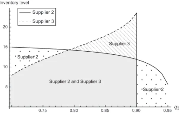
Figure 4 shows how the optimal threshold value changes as a function of the probability of reliability for demand node 3 and Figure 5 shows how the order quantity changes as the probability of reliability changes. As the probability of reliability increases at supply node 3, the order quantity of this supply node 3 increases as well.
Since the threshold of node 3 is larger than that of node 2 for q3 ≥ 0.8 in Figure 4,
goods are only shipped from supply node 3 when the inventory level is at a moderate level because the production cost of supplier 3 is lower than that of supplier 2∥. However, when the probability of reliability at node 3 is smaller than q3 = 0.8, goods are only shipped from
supply node 2 due to low probability of reliability at node 3∗∗. It is optimal to supply from node 2 and 3 when the inventory level lies in the gray area of Figure 4.
Figure 6 and Figure 7 show how the optimal threshold level and order quantity change as a function of the demand risk at node 2 (σ2). Figure 6 tells us inventory level increases as σ2 increases for supply node 3, but the inventory level decreases as σ2 increases for supply
node 2. This occurs because supply node 3 serves as the main supplier (i.e. risk adjusted cost index is larger). Figure 7 tells us that when demand risk is high, the order quantity increases for supply node 3 which has a smaller production cost, and the order quantity decreases for supply node 2 which has a higher production cost. This means that when the demand risk is high, the procurement is based on the supplier that has a lower production cost/lower reliability.
∥Shaded area in Figure 4. This corresponds to the second case in equation (4.11). ∗∗Dotted area in Figure 4. This corresponds to the second case in equation (4.12).
Supplier 2 Supplier 3
Inventory level
Supplier 3
Supplier 2 and Supplier 3 Supplier 2
Supplier 2
Figure 4: The optimal policy threshold as a function of the probability of reliability at supply node 3
Order quantity
Supplier 2 Supplier 3
Figure 5: The optimal order quantity as a function of the probability of reliability at supply node 3
Supplier 2 Supplier 3 Inventory level
Supplier 3
Supplier 2 and Supplier 3
Figure 6: The optimal policy threshold as a function of the demand risk at supply node 2
Supplier 2
Order quantity
Supplier 3
Figure 7: The optimal order quantity as a function of the demand risk at supply node 2
5. Multiperiod Model
5.1. The formulation of the multiperiod model
This section extends the single period model to a multiperiod model in discrete time where the time to the planning horizon t is t = 0, 1, ..., T , i.e. t = 0 is the last period and t = T corresponds to the first period. If the state is i at the beginning of period t, the inventory level of the demand node is y, and the order quantity is s, the total expected cost function becomes vt(i, s, y) = J (i, s, y) + ∑ i̸=j Pij(t− 1)hN + Kt(i, s, y), (5.1) Kt(i, s, y) = N ∑ j=1 Pij(t− 1)E[Vt−1(j, y + C ′ (i)(R· s) − D(i))], (5.2)
where function J is the one period total cost function given by equation (4.1) and R ∈ RKi.
hN ≥ 0 is the cost to switch the supply chain network in state N, the second term in function
K is the minimum total expected cost beyond period t− 1. Thus, the order quantity that
minimizes the total expected cost becomes the optimal policy:
Vt(i, y) = min
where V0(i, y) = 0.
Lemma 5.1. For fixed i and t, we have
(i) vt(i, s, y) is convex in (s, y).
(ii) Vt(i, y) is convex in y.
Proof. The proof for this lemma follows the proof of Lemma 4 in Gallego and Hu [2]. The
proof is by induction on t. For t = 1, the assertions clearly hold. We assume for t− 1. By Lemma 4.1, since vt−1 is convex, Kt(i,·, ·) is convex in (s, y). Thus, vt(i,·, ·) is convex in
(s, y).
Lemma 5.2. Suppose that Assumptions 3.1, 4.1 and 4.2 hold. For any l = 1, ..., L and
k ∈ Ki
I(l), there exists a unique value ˜yl(t, i, k) such that
Φsk(t, i, sl, ˜yl(t, i, k))|sk=0 = 0, (5.3)
where Φsk(t, i, s, yl) ≡ ∂vt(i, sl, y)/∂sk, and, for k1, k2 ∈ K
i
II(l), there exist values (˜yl(t, i, k1), ˜yl(t, i, k2)) where ˜yl(t, i, k1) is satisfying
Φsk1(t, i, sl, ˜yl(t, i, k1))|sk1=0 = Φsk2(t, i, sl, ˜yl(t, i, k2))|sk1=0 = 0. (5.4)
and ˜yl(t, i, k2) is satisfying
Φsk1(t, i, sl, ˜yl(t, i, k1))|sk2=0 = Φsk2(t, i, sl, ˜yl(t, i, k2))|sk2=0 = 0.
Proof. For k∈ KiI(l), from equation (4.6), we obtain
Φsk(t, i, s, yl)|sk=0 = ck− plqk+ (hl+ pl)Fi,l(yl) + Ξsk(t, i, s, yl)|sk=0,
where Ξsk(t, i, sl, yl)≡ ∂Kt(i, s, y)/∂sk. From equation (5.2), we have
Ξsk(t, i, sl, yl) = N ∑ j=1 Pij(t− 1) { ∂ ∂sk E[J (j, ˆsj, y)] + ∂ ∂sk E[Kt−1(j, ˆsj, y)] } ,
where y ≡ y + C′(i)(Ri· si)− Di. Here, we have ∂ ∂sk E[J (j, ˆsj, y)] = E [ ∂ ∂sk J (j, ˆsj, y) ] = E [ ∂ ∂ylJ (j, ˆs j, y)∂yl ∂sk ] = E[{(hl+ pl)Fi,l(yl+ Bl(ˆsj))− pl}Rk]
where yl is the lth component of the vector y, that is, yl = yl +
∑Ki u=1Cul(i)Rusu − Dl. Thus, we have lim yl→+∞ ∂ ∂sk E[J (j, s∗j, y)] sk=0 = hlqk. So, we obtain lim yl→+∞ Ξsk(t, i, sl, yl)|sk=0= hlqk+ lim yl→+∞ N ∑ j=1 Pij(t− 1) ∂ ∂sk E[Kt−1(j, ˆsj, y)] sk=0 .
By applying the argument above repeatedly, we obtain lim yl→+∞ Ξsk(t, i, sl, yl)|sk=0= (t− 1)hlqk. (5.5) Thus, we have lim yl→+∞ Φsk(t, i, sl, yl)|sk=0= ck+ thlqk > 0. Similarly, we have lim yl→−∞ Φsk(t, i, sl, yl)|sk=0= ck− tplqk < ck− plqk< 0.
Thus, there exists ˜yl(t, i, k), k ∈ KiI(l), satisfying equation (5.3). To show that ˜yl(t, i, k), k ∈ KIi(l), is unique, suppose there exists ˜yl1 < ˜yl2 such that
Φsk(t, i, sl, y 1
l)|sk=0= Φsk(t, i, sl, y 2
l)|sk=0= 0. (5.6)
For ˜yl2 > 0, we have Fi,l(˜y2l) > Fi,l(˜yl1). It follows from equation (4.6) that Θsk1(i, s, ˜yl2)|sk=0
> Θsk1(i, s, ˜yl1)|sk=0. Since the function Vt−1(i,·) is convex in y by the induction hypothesis,
∂Vt−1(i,·)/∂yl is increasing in yl. Thus, Ξsk(t, i, sl, yl) is also increasing in yl which implies
Φsk(t, i, sl, y 1
l)|sk=0< Φsk(t, i, sl, y 2
l)|sk=0 .
This is a contradiction to equation (5.6). For ˜y2
l ≤ 0, we have Fi,l(˜y1l) = Fi,l(˜yl2) = 0. Thus,
we have Θsk1(i, sl, yl1) |sk=0= Θsk1(i, sl, yl2) |sk=0= ck − plqk. Since Φsk(t, i, sl, yl) |sk=0=
Θsk(i, sl, yl)|sk=0+Ξsk(t, i, sl, yl)|sk=0, the first equality of equation (5.6) is equivalent to
Ξsk(t, i, sl, y 1
l) = Ξsk(t, i, sl, y 2
l) = plqk− ck > 0.
Hence, this is a contradiction to equation (5.6).
For k1, k2 ∈ KiII(l), by equations (4.7) and (4.8), we obtain
Φsk1(t, i, sl, yl)|sk1=0 = ck1 − plqk1 + (hl+ pl){qk1qk2Fi,l(yl+ sk2)
+qk1(1− qk2)Fi,l(yl)} + Ξsk1(t, i, sl, yl)|sk1=0= 0, (5.7) Φsk2(t, i, sl, yl)|sk1=0 = ck2 − plqk2 + (hl+ pl)qk2Fi,l(yl+ sk2)
+Ξsk2(t, i, sl, yl)|sk1=0= 0. (5.8)
Substituting equation (5.7) into equation (5.8), we have A1(yl) = 0, where A1(yl)≡ ck1 − ck2qk1 − plqk1(1− qk2) + (hl+ pl)qk1(1− qk2)Fi,l(yl)
+ Ξsk1(t, i, sl, yl)|sk1=0 −qk1Ξsk2(t, i, sl, yl)|sk1=0 . (5.9) We will show the existence of a value ˜yl satisfying A1(˜yl) = 0. From equation (5.5), we
obtain
lim
yl→+∞
A1(yl) = ck1 − ck2qk1 + thlqk1(1− qk2) > 0. The last inequality follows from Assumption 4.1. Similarly, we have
lim
yl→−∞
The last inequality follows from Assumption 4.2. Thus, there exists ˜yl(t, i, k), k ∈ KiII(l),
satisfying equation (5.4) (that is, A1(˜yl) = 0). To show that ˜yl(t, i, k) is unique, suppose
there exist ˜y1 l < ˜yl2 such that A1(y1l) = A1(y2l) = 0. (5.10) Here, we have Ξsk1(t, i, sl, yl)|sk1=0− qk1Ξsk2(t, i, sl, yl)|sk1=0 = N ∑ j=1 Pi,j(t− 1)E [ ∂Vt−1(j, y) ∂sk1 − qk1 ∂Vt−1(j, y) ∂sk2 ] = N ∑ j=1 Pi,j(t− 1)E [ qk1 ∂Vt−1(j, y) ∂y − qk1qk2 ∂Vt−1(j, y) ∂y ] = qk1(1− qk2) N ∑ j=1 Pi,j(t− 1)E [ ∂Vt−1(j, y) ∂y ] .
Thus, from Lemma 5.1(ii), Vt−1(j, y) is convex in yl, and so A1(yl) is also increasing in yl.
Hence, there exists a value ˜yl(t, i, k1) such as Φsk1(t, i, sl, ˜yl)|sk1=0 = 0. Similarly, we can
also show the existence of ˜yl(t, i, k2) satisfying equation (5.4) by setting sk2 = 0. In other words, ˜yl(t, i, k2) can be obtained as a solution to A2(˜yl) = 0, where
A2(yl)≡ ck2 − ck1qk2 − plqk2(1− qk1) + (hl+ pl)qk2(1− qk1)Fi,l(yl)
+ Ξsk2(t, i, s, yl)|sk2=0 −qk2Ξsk1(t, i, s, yl)|sk2=0 . (5.11)
Lemma 5.3. When ck2/qk2 ≤ (≥)ck1/qk1, we have ˜yl(t, i, k1)≤ (≥)˜yl(t, i, k2).
Proof. By equation (5.9), we have A1(˜yl(t, i, k1)) = 0, that is,
qk1(1− qk2){pl− (hl+ pl)Fi,l(˜yl)− M(˜yl)} = ck1 − ck2qk1,
where M (y) = ∑Nj=1Pi,j(t − 1)E[∂Vt−1(i, y)/∂y]. Substituting the above equation into
equation (5.11), we have
A2(˜yl(t, i, k1)) = ck2 − ck1qk2 − qk2(1− qk1){pl− (hl+ pl)Fi,l(˜yl(t, i, k1))− M(˜yl(t, i, k1))} = 1− qk1qk2
qk1(1− qk2)
(qk1ck2 − qk2ck1).
Thus, if ck2/qk2 ≤ (≥)ck1/qk1, we have A2(˜yl(t, i, k1))≤ (≥)A1(˜yl(t, i, k1)) = 0. Since A1(yl) and A2(yl) are increasing in yl, we obtain ˜yl(t, i, k1)≤ (≥)˜yl(t, i, k2).
Lemma 5.4. Suppose that Assumptions 3.1, 4.1 and 4.2 hold. For fixed t and yl, when
k ∈ Ki
I(l), there exists a value ˆsk(t, i, yl) such that Φsk(t, i, sl, yl) = 0. Moreover, when k ∈
Ki
II(l), there exist a value (ˆsk1(t, i, yl),ˆsk2(t, i, yl)) such that Φsk1(t, i, sl, yl) = Φsk2(t, i, sl, yl) = 0.
Proof. For k∈ Ki
I(l), we have Φsk(t, i, s, yl)→ ck+ qkhlt > 0 as sk→ +∞ and Φsk(t, i, s, yl)
→ ck− qkplt < 0 as sk → −∞. By induction, Φsk(t, i, sl, yl) is increasing in sk. Thus, there
exists a value ˆsk(t, i, yl).
For k ∈ Ki
II(l), from equations Θsk1(i, sl, yl) = 0 and Θsk2(i, sl, yl) = 0, we obtain B(sk1, sk2) = 0, where
Bi,l(sk1, sk2) ≡ Θsk1(i, sl, yl)− Θsk2(i, sl, yl) = ck1 − ck2 − pl(qk1 − qk2) +(hl+ pl){qk1(1− qk2)Fi,l(yl+ sk1)− qk2(1− qk1)Fi,l(yl+ sk2)} +(qk1 − qk2) N ∑ j=1 Pi,j(t− 1)E [ ∂Vt−1(j, y) ∂y ] .
For given sk2, we have
∂Bi,l ∂sk1 = (hl+ pl)qk1(1− qk2)fi,l(yl+ sk1) + qk1(qk1 − qk2) N ∑ j=1 Pi,jE [ ∂2Vt−1(j, y) ∂y2 ] ≥ 0.
The last inequality follows from the convexity of Vt−1(j,·). As sk1 → +∞, we have
Bi,l(sk1, sk2) = ck1− ck2 − pl(qk1 − qk2) +(hl+ pl){qk1(1− qk2)− qk2(1− qk1)Fi,l(yl+ sk2)} +(qk1 − qk2)(t− 1)hlqk1 ≥ ck1− ck2 + hl(qk1 − qk2)(1 + (t− 1)qk1) ≥ 0. In addition, as sk1 → −∞, we have Bi,l(sk1, sk2) = ck1 − ck2 − pl(qk1 − qk2) −qk2(hl+ pl)(1− qk1)Fi,l(yl+ sk2)− (qk1 − qk2)(t− 1)qk1pl ≤ 0
Thus, for given sk2, there exists a unique ˆsk1 such that Bi,l(sk1, sk2) = 0. Similarly, for given
sk1, we can show that there exists a value ˆsk2. Hence, there exists a pair (ˆsk1,ˆsk2) satisfying Φsk1(t, i, sl, yl) = Φsk2(t, i, sl, yl) = 0.
Theorem 5.1. Suppose that Assumptions 3.1, 4.1 and 4.2 hold. (i) When the state is i and
the inventory level of demand point l is yl, the optimal order quantity for supplier k∈ KiI(l)
is given by ˜ sk(t, i, yl) = { ˆ sk(t, i, yl), if yl< ˜yl(t, i, k), 0, if yl≥ ˜yl(t, i, k).
(ii) When the state is i and the inventory level of demand point l is yl, if ck2/qk2 ≤ ck1/qk1,
then the optimal order quantity for supplier k1, k2 ∈ KiII(l) is given by
{˜sk1(t, i, yl), ˜sk2(t, i, yl)} = {ˆsk1(t, i, yl), ˆsk2(t, i, yl)}, if yl < ˜yl(t, i, k1), {0, ˆsk2(t, i, yl)}, if ˜yl(1, i, k1) < yl < ˜yl(t, i, k2), {0, 0}, if ˜yl(t, i, k2) < yl.
and if ck1/qk1 ≥ ck2/qk2, we have {˜sk1(t, i, yl), ˜sk2(t, i, yl)} = {ˆsk1(t, i, yl), ˆsk2(t, i, yl)}, if yl < ˜yl(t, i, k2), {ˆsk1(t, i, yl), 0}, if ˜yl(1, i, k2) < yl < ˜yl(t, i, k1), {0, 0}, if ˜yl(t, i, k1) < yl.
Proof. The proof directly follows from Lemma 5.1-5.4.
We see that the structure of the optimal policy for the multiperiod case is the same as that for the single-period case.
Next, we show the monotonicity of the expected cost function for the multi period case. Here, we assume that a finite Markov chain X is a homogeneous Markov process with state space S = {1, .., N}. Let Pi,j denote the transition probability that satisfies the following
assumption.
Assumption 5.1. For each k ∈ S, ∑Nj=kPi,j is non-decreasing in i.
Definition 5.1 (M¨uller and Stoyan [9], p.98). Let X and Y be n-dimensional random
vectors with finite expectations. Then we say that
(i) X is less than Y in convex order (written X ≤cx Y ), if E[f (X)] ≤ E[f(Y )] for all
convex functions f :Rn→ R such that the expectations exist.
(i) X is less than Y in increasing convex order (written X ≤icx Y ), if E[f (X)]≤ E[f(Y )]
for all increasing convex functions f :Rn→ R such that the expectations exist.
Proposition 5.1. Suppose that Assumption 5.1 holds.
(i) Define O(i) ≡ C′(i)(R · s). For any l and i ≤ i′, i, i′ ∈ S, if D(i) ≤cx D(i
′ ) and O(i)≤cx O(i ′ ), then Vt(i,·) ≤ Vt(i ′ ,·).
(ii) For any k, if pl= 0 and ˆR≤icxR, then Vt(i,· : ˆR)≤ Vt(i,· : R).
Proof. By equation (5.1), for i≤ i′, we have
vt(i, s, y) = J (i, s, y) + ∑ i̸=j PijhN + N ∑ j=1 PijE[Vt−1(j, yi)], ≤ J(i, s, y) +∑ i̸=j PijhN + N ∑ j=1 PijE[Vt−1(j, yi′)], ≤ J(i′, s, y) +∑ i̸=j Pi′jhN + N ∑ j=1 Pi′jE[Vt−1(j, yi′)], = vt(i ′ , s, y),
where y = y + C′(i)(R·s)−D(i). The first inequality follows from the convexity of Vt(i, y)
with respect to y given in Lemma 5.1(ii). The second inequality is obtained by the proof of Proposition 4.1(ii) and Assumption 5.1. This result leads to the assertion. Similarly, we can show part (ii) by the convexity of Vt(i, y) with respect to y.
5.2. Numerical example
This section examines how network flexibility impacts the total expected cost by numerically analyzing a supply chain consisted of 3 supply nodes and 2 demand nodes (e.g. Figure 1
and Figure 2), The planning horizon is set to T = 3 and the inventory level at the beginning of time period 3 is y1 = y2 = 0, and the transition probability matrix is given as
P = ( 0.8 0.2 0.3 0.7 ) .
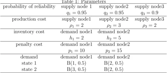
The transportation cost is set to a = 0. Although there are no particular distribution assumptions required for the demand distribution, for numerical illustration, we assume that demand Dl(i) follows a binomial distribution with parameters in Table 1. The binomial
distribution will be denoted as B(trials, successes). In order to evaluate the performance of flexibility residing in the supply chain network, we will compare the following two cases. The first case will apply the network for state 1 regardless of the realized state of supply (no switching in the network). The second case switches the network depending on the state of the supply such that the total cost is minimized. In both cases, the demand will follow a probability distribution that depends on the state of the network.
Figure 8 shows the minimum total cost for the planning horizon, i.e. 3 periods, when the disruption probability q1is set to 0.9−0.99. Here, the bold line and dotted line represent the
switching case and no switching case, respectively. For each case, there are two lines with a different initial state for the planning horizon (i.e. the beginning of the 3rd period). When there is no switching in the network, the disruption in supply node 1 completely stops the supply to demand node 1. Thus, as the disruption probability increases (i.e. q1 decreases),
the cost increases. Accordingly, when the network is in state 2, demand node 1 receives supply from supply node 1 and supply node 2 simultaneously. As a consequence, when there is switching in the network, the total cost is smaller than the case for no switching, i.e. the cost becomes smaller. In addition, Figure 9 illustrates the percentage of cost of switching the network compared to the cost of non-switching. Since the cost improvement is positive regardless of the network state and disruption probability, we can say that the flexibility in supply reduces the total expected cost when disruption probability is present.
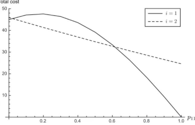
Figure 10 compares the minimum total cost when the transition probability from state 1 to state 1 is altered. We can easily observe that when the transition probability p11 is
smaller, the state of market demand is more likely to shift from state 1 to state 2. By observing the dotted lines, the cost increases if market demand is more likely to shift to state 2 (i.e. p11 is smaller) when there is no switching in the supply chain network. This
phenomenon occurs because the demand variance of demand node 1 in state 2 is larger than that of state 1. Figure 11 shows the cost improvement by flexibility. When the initial state is in state 1, the effect of flexibility on the improvement is lower as the possibility of remaining in state 1 becomes higher. However, we can say that the network switching is effective in a case when the demand environment is more volatile.
6. Conclusion
This paper explicitly models disruption probability in the supply chain with state dependent uncertain demand. We derive an optimal threshold policy when there are two supply nodes and one demand node that needs multiple products. The policy is derived for the single period case and multiperiod case, and in addition, we show that the expected cost function is monotonic in the convex ordering of the demand distribution. The results differ from the past literature in the sense that we deal with the disruption probability via altering the state dependent supply chain network, and derive the optimal threshold policy.
The contribution of this paper lies in showing a general direction to corporations that may need to diversify their production facilities by modifying their supply chain network.
Table 1: Parameters
probability of reliability supply node 1 supply node2 supply node3
q1 = 0.95 q2 = 0.95 q3 = 0.9
production cost supply node1 supply node2 supply node3
ρ1 = 2 ρ2 = 3 ρ3 = 2
inventory cost demand node1 demand node2
h1 = 2 h2 = 5
penalty cost demand node1 demand node2
p1 = 10 p2 = 15
demand demand node1 demand node2
state 1 B(1, 0.5) B(2, 0.5)
state 2 B(3, 0.5) B(2, 0.5)
The numerical examples show that the potential improvement of the total expected cost may run up to 17% to 30% depending on the parameters. This numerically verifies the results of our theorems and justifies the importance of using our proposed model when introducing flexibility in the supply chain.
We believe this model can cope with the practical needs of corporations because of its simplicity. The supply chain disruptions cause the network configuration to become state dependent, which significantly reduces the number of situations to be considered. In addition, the risk adjusted cost index provides a good indicator on how to switch suppliers to fulfill the unmet demand.
References
[1] A. Federgruen and P. Zipkin: Approximations of dynamic multilocation production and inventory problems. Management Science, 30 (1984), 69–84.
[2] G. Gallego and H. Hu: Optimal policies for production/inventory systems with finite capacity and Markov-modulated demand and supply processes. Annals of Operations
Research, 126 (2004), 21–41.
[3] Y. Gerchak and M. Parlar: Yield variability, cost tradeoffs and diversification in the EOQ model. Naval Research Logistics, 37 (1990), 341–354.
[4] D. Gupta and W.L. Cooper: Stochastic comparisons in production yield management.
Operations Research, 37 (1990), 341–354.
[5] D.P. Heyman and M.J. Sobel: Stochastic Models in Operations Research, Vol. 2 (New York: McGraw-Hill, 1984).
[6] W.C. Jordan and S.C. Graves: Principles on the benefits of manufacturing flexibility.
Management Science, 41-4 (1995), 577–594.
[7] S. Kunnumkai and H. Topaloglu: Approximate dynamic programming methods for an inventory allocation problem under uncertainty. Naval Research Logistics, 53 (2006), 822–841.
[8] S. Kunnumkai and H. Topaloglu: A duality -based relaxation and decomposition ap-proach for inventory distribution systems. Naval Research Logistics, 55 (2008), 612–631. [9] A. M¨uller and D. Stoyan: Comparison Methods for Stochastic Models and Risks (Wiley
Series in Probability and Statistics. John Wiley & Sons Ltd., Chichester, 2002). [10] S. Saghafian and M.P. Van Oyen: Compensating for dynamic supply disruptions:
[11] H. Sak and C¸ . Haks¨oz: A copula-based simulation model for supply portfolio risk.
Journal of Operational Risk, 6-3 (2011), 15–38.
[12] A.J. Schmitt and L.V. Snyder: Infinite-horizon models for inventory control under yield uncertainty and disruptions. Computers & Operations Research, 39 (2012), 850–862. [13] L.V. Snyder, Z. Atan, P. Peng, Y. Rong, A.J. Schmitt, and B. Sinsoyasal: OR/MS
models for supply chain disruptions: a review. IIE Transactions, 48 (2016), 89–109. [14] S.C. Tang: Perspectives in supply chain risk management. International Journal of
Production Economics, 103 (2006), 451–488.
[15] S.C. Tang: Robust Strategies for mitigating supply chain disruptions. International
Journal of Logistics Research Applications, 9 (2006), 33–45.
[16] J.A. Van Mieghem: Investment strategies for flexible resources. Management Science,
44-8 (1998), 1071–1078.
Flexible SC Fixed SC
Total cost
Figure 8: Reliability probability at supply node 1 and minimum total expected cost
Figure 9: Reliability probability at supply node 1 and improvement due to flexibility
Flexible SC Fixed SC
Total cost
Figure 10: Transition probability from state 1 to state 1 and minimum total expected cost
Total cost
Figure 11: Transition probability from state 1 to state 1 and improvement due to flexi-bility
Kimitoshi Sato Kanagawa University Faculty of Engineering
3-27-1 Rokkakubashi, Kanagawa-ku, Yokohama, Kanagawa 221-8686, Japan E-mail: [email protected]