An Efficient Vector Transfer for Sparse Matrix-Vector Multiplication on Distributed Memory Systems

全文

(1)Vol.2010-HPC-124 No.9 2010/2/22 IPSJ SIG Technical Report. into submatrices and subvectors to make each of them reside in a portion of distributed memory and thus to assign the computation of a submatrix and subvectors to the process corresponding to the memory portion. For example, a row-wise block-decomposition assigns a set of contiguous rows of A to a process which should naturally have the corresponding part of the product vector w. The process may also have a part of the multiplier vector v rather than the whole of it exploiting the sparseness of the matrix A. That is, the process only requires a part of components of v which corresponds to the non-zero entries of A. The problem in giving a process its necessary components of v is that the components can be distributed in many processes because a component is usually derived from the corresponding component of w by the process having it. A simple but spatially and temporally inefficient solution is to use an all-gather type communication so that every process is given the whole of v regardless of its necessity. More sophisticated and efficient solution is to analyze the matrix A prior to the iterative multiplications to have a kind of flow graph representing every sender/receiver pair for each subset of v’s components which the receiver requires and the sender has. Since the v’s components which a receiver needs are not necessary to be contiguous but may form a set of fragments, we have to determine how a sender sends the fragments to the receiver. A simple way is to send each fragment individually potentially causing a flood of small messages. Another simple tactics is to pack the components into a buffer for sending to minimize the number of messages paying the cost of copying. In addition, we found the third option in which fragments are combined together with the gaps between them to form a large message without copying. Since the message transfer time with each of three tactics above depends on the number of fragments and the size of each fragment and each gap, the best solution is an assortment of the tactics applied to sets of fragments. For example, the individual sending will be apply to large fragments, while packing and combining should have advantage for a series of smaller fragments separated by large and small gaps respectively. Our primary contribution described in this paper is the proposal of an algorithm based on dynamic programming to find the optimum assortment, which is. An Efficient Vector Transfer for Sparse Matrix-Vector Multiplication on Distributed Memory Systems Hiroshi Nakashima,†1 Toshiyuki Fukuhara†2 and Takeshi Iwashita†1 This paper proposes an efficient algorithm to exchange fragments of a vector distributed among processes which repeatedly perform sparse matrix-vector multiplication in parallel and in a block-decomposed manner. The idea to reduce the communication cost for the exchange is to combine non-contiguous fragments of a vector residing in a process and required by another process to multiply the fragments by the submatrix in the receiver process. That is, the sender may send fragments and gaps between them forming a larger fragment, rather than sending each fragment individually or packing fragments into a single vector before sending. The key feature of our algorithm is to find the optimum assortment of combining, individual sending and packing based on dynamic programming from given fragments and non-linear cost functions. Our preliminary evaluation with artificially generated sparse matrices shows the optimum assortment is up to 1.5 times as fast as simple packing.. 1. Introduction Sparse matrix-vector multiplication is a frequently used kernel operation in numerical and scientific programs including those implementing iterative methods to solve linear equations and to find eigenvalues. These iterative methods typically repeats wi+1 = Av i with a fixed sparse matrix A and vectors v i and wi+1 from which the multiplier vector of the next iteration step v i+1 is derived. Parallelizing the programs and methods with sparse matrix-vector multiplication of large dimension is inevitable not only to accelerate them but also to simply accommodate the large size matrices and vectors in a computing system. The latter requirement usually leads us to decompose the matrix and vectors †1 ACCMS, Kyoto University †2 Graduate School of Informatics, Kyoto University. 1. c 2010 Information Processing Society of Japan ⃝.

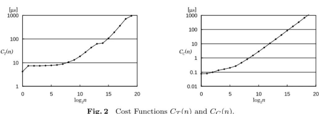
(2) Vol.2010-HPC-124 No.9 2010/2/22 IPSJ SIG Technical Report. discussed in Section 3 after we define the problem more formally in Section 2. The implementation of the algorithm and its performance are then shown in Section 4. Finally we conclude the paper in Section 5.. A. 2. Problem Definition. A1. v1. A2. v2 ×. Let A be a sparse square matrix of N × N having entries a(i, j) (i, j ∈ [1, N ]), and v be a N -dimensional vector having components v(i) (i ∈ [1, N ]). Then A and v are decomposed into P submatrices and subvectors as     A1 v1  .   .  A =  ..  v =  ..  (1) AP. V 32. v. A3. v3. A4. v4. 33 f(1) h(1)=34 s(1)=3. vP. 48 f(2) h(2)=40 s(2)=4. f(3) h(3)=46 s(2)=2. F(1,2) F(2,3) F(3,4) + + F(1,3) F(3,4) + F(3,4) F(1,3) + F(1,2) F(2,4) + F(1,2) F(2,4) + F(1,4) F(1,4). so that each submatrix Ap having Np rows and Np -dimensional subvector vp are assigned to the process p ∈ [1, P ] (see Fig. 1). A process p performs a part of the matrix-vector multiplication w = Av, namely wp = Ap v to produce the Np -dimensional subvector wp of the product vector w. For this operation, the process p needs a set of components of v namely ∑p−1 Vp = {v(i) | a(i, j) ̸= 0, Kp < i ≤ Kp+1 , 1 ≤ j ≤ N } where Kp = q=0 Np . The component set Vp is divided into disjunct subsets Vp1 , . . . , VpP such that Vpq = {v(i) ∈ Vp | Kq < i ≤ Kq+1 } to form the set of components to be sent from the process q to p. Now let us concentrate on the sender/receiver process pair q and p to simplify the notations and let V = Vpq . Let I be the set of indices of the components in V , i.e., I = {i | v(i) ∈ V }. The ascendingly ordered sequence i1 , . . . , ik (k = |I|) of indices in I is divided into disjunct index fragments ϕ(1), . . . , ϕ(m) such that ∪m I = j=1 ϕ(j) and each of them has contiguous indices. That is, each ϕ(j) satisfies the followings where h(j) = min ϕ(j) and s(j) = |ϕ(j)|. ∀i ∈ ϕ(j) : h(j) ≤ i < h(j) + s(j) (2) ∀j ∈ [1, m−1] : h(j) + s(j) < h(j + 1) (3) Then, with each index fragment ϕ(j), we define the fragment of vector components f (j) = {v(i) | i ∈ ϕ(j)}. Vector components in a contiguos sequence of fragments, or chunk, from f (j). Fig. 1 Example of A × v, fragments, chunks and assortments. ∪k−1 to f (k − 1), i.e., F (j, k) = l=j f (l) can be transferred from the process q to p as a single message by one of the following ways. One way is to pack them into ∑k−1 a message buffer of l=j s(l) components and send the contents of the buffer minimizing the message size while paying the cost of copying. The other way is to combine the fragments without copying to have a message including not only them but gaps between them, making message size h(k − 1) + s(k − 1) − h(j) larger than required. The cost to transfer a fragment or a chunk is defined as follows. Let CT (n) be the non-decreasing function of n to give the time to transfer a message having n vector components from q to p, and CC (n) be that to give the time to copy n contiguous components from the vector store to the buffer for packing. With these cost functions, we can define the costs of the packing and combining transfer of a chunk F (j, k) from q to p, namely Cpack (j, k) and Ccomb (j, k) as follows.   k−1 k−1 ∑ ∑ Cpack (j, k) = CT  s(i) + CC (s(i)) (4) i=j. i=j. Ccomb (j, k) = CT (h(k − 1) + s(k − 1) − h(j)). 2. (5). c 2010 Information Processing Society of Japan ⃝.

(3) Vol.2010-HPC-124 No.9 2010/2/22 IPSJ SIG Technical Report. Note that the second term of the equation (5) above is the sum of copying costs of the fragments rather than the cost for the sum of fragment sizes, because we have to take care of the overhead incurred in each fragment copy. Then C(j, k) = min(Cpack (j, k), Ccomb (j, k)) gives us the cost to send F (j, k) as a single message. Note that C(j, j+1) = Ccomb (j, j+1) = CT (s(j)) is the transfer ∑k−1 cost of the single fragment f (j), and their sum over F (j, k), i.e., i=j C(i, i + 1) can be smaller than C(j, k). In general, the minimum transfer cost for a fragment sequence is given by a series of packing/combining transfers of its subsequences, i.e., chunks. Now we define our problem as follows: from a given fragments f (1), . . . , f (m), find the set of chunks F (j1 , j2 ), . . . , F (jn , jn+1 ), or the assortment of the fragments, where j1 = 1, jn+1 = m + 1, and ji < ji+1 for all i ∈ [1, n], such that ∑n i=1 C(ji , ji+1 ) is minimized.. based on dynamic programming technique. for k = 1 to m do Cmin (1, k ) ← C (1, k ); for n = 2 to m do begin for k = n to m do begin cmin ← Cmin (n − 1, k ); jmin ← k ; for j = k − 1 downto n − 1 do begin c = Cmin (n − 1, j ) + C (j , k ); if c < cmin then begin cmin ← c; jmin ← j ; end end Cmin (n, k ) ← cmin ; Jmin (n, k ) ← jmin end end. 3. Algorithm To solve the minimization problem defined in the previous section, we introduce a subproblem defined as follows. { n }

(4) ∑

(5)

(6) Cmin (n, k) = min C(ji , ji+1 )

(7) j1 = 1, jn+1 = k + 1, ji ≤ ji+1 (6) j2 ,...,jn. The code above give us the optimum assortment of fragments by a sequence of their indices j2 , . . . , jm which minimize the right-hand side of the equation (6) for Cmin (m, m), i.e., the arg min of the equation, through a back-trace of Jmin (n, k) as follows. jm = Jmin (m, m) jn = Jmin (n, jn+1 ) (2 ≤ n < m) (8) It is clear that the code above takes O(m3 ) time providing that we can calculate C(j, k) in the most-inner loop in O(1) time for each. From equations (4) ∑k−1 and (5), an O(1) calculation is easily implemented by keeping track i=j s(i) ∑k−1 and i=j CC (s(i)). As for the spatial complexity, it is also obvious we need O(m2 ) space to keep Jmin (n, k)⋆1 .. i=1. The cost Cmin (n, k) above means the minimum transfer cost for fragments f (1), . . . , f (k) with at most n chunks which are F (ji , ji+1 ) with all ji such that i ∈ [1, n] to give the minimum but excluding those ji = ji+1 because F (ji , ji ) means a empty chunk by definition and thus C(ji , ji ) = 0. It is clear that Cmin (1, k) = C(1, k) from the definition above, and also that Cmin (m, m) gives the minimum cost for the original problem. Since C(ji , ji+1 ) can be calculated from any other C(ji′ , ji′ +1 ), the definition above can be rewritten with the formulation similar to that presented in Ref. 1) as follows. Cmin (n, k) = min {Cmin (n − 1, j) + C(j, k)} 1≤j≤k. 4. Experiments 4.1 Implementation and Evaluation Environment We implemented the algorithm discussed in Section 3 together with the vector transfer for multiplying it to a sparse matrix represented in CRS format, using. (7). ⋆1 It is unnecessary to have Cmin (n, k) for all n ∈ [1, m] because only Cmin (n−1, k) is required to calculate Cmin (n, k), and thus the space for it is O(m). The O(m2 ) for Jmin (n, k), on the other hand, is essential.. From the recurrence above and the obvious facts that Cmin (n, k) = Cmin (k, k) for any n > k and C(j, j) = 0 for any j by definition, we have the following code. 3. c 2010 Information Processing Society of Japan ⃝.

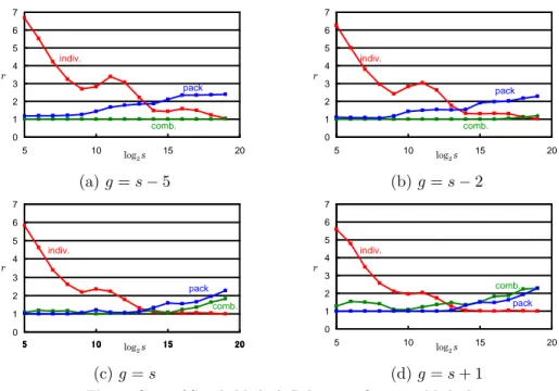
(8) Vol.2010-HPC-124 No.9 2010/2/22 IPSJ SIG Technical Report [µs] 1000. [µs] 1000. each. That is, we ran simple measurement programs using Fujitsu’s C compiler version 3.0 and MPI library version 3.0, which are also used for the main program and its evaluation, to obtain the performance data shown in Fig. 2 for n = 2i vector components where i ∈ [0, 19]. Then each cost function with n components looks the table of performance data by l = ⌊log2 n⌋ and l + 1 to have the linearly interpolated value for n by;  l+1  − n)Cx (2l ) + (n − 2l )Cx (2l+1 )  (2 n ≤ 219 l 2 Cx (n) ≈ n   Cx (219 ) n > 219 219. 100 100. 10 CC(n) 1. CT(n) 10. 0.1 1. 0.01 0. 5. 10 log2n. 15. 20. 0. 5. 10 log2n. 15. 20. Fig. 2 Cost Functions CT (n) and CC (n).. for Cx (n) ∈ {CT (n), CC (n)}. 4.2 Cost Optimality The first experiment is to evaluate how small cost the optimum assortment gives compared to other simple methods. That is, we evaluated the costs of transferring ten fragments of various sizes and gaps between them with the following four methods; individual, packing and combining methods which sends all fragments individually, packing them into one message, and combining them and gaps to form one message, while optimum is our proposed one. We evaluated the amount of the cost using the cost functions rather than measuring the time for vector transfers. Therefore, the evaluation gives how our optimum method works well theoretically. Fig. 3 shows normalized costs r relative to the optimum ones for randomly generated fragments having 2s vector components on average, and 2g components in each gap on average. Graphs in the figure are for the cases of g ∈ {s−5, s−2, s, s+1}, while s is varied from 5 to 19 in each case. Each value shown in the graphs is the average of ten experiments with specific settings of s and g. It is observed from the graphs that the individual method incurs high costs when the size of fragments and gaps is small but becomes optimum when the size increases as easily expected. As for other two simple methods to send all fragments by one message, one of them is almost optimum for small size fragments but it depends on the gap size which method is better and (nearly) optimum. On the other hand, the optimum method gives not only the best of three simple. C99 and MPI-2.0. The program consists of the following two procedures. • A scheduler in which each process p analyzes the given submatrix Ap to find the optimum assortments for all v q which the process requires for the multiplication with Ap . Then all processes perform an all-to-all type communication to exchange the assortments so that each process p has assortments of v p to send its components to other processes. In addition, the submatrix Ap is transformed into A′p so that its entry a′ (i, j ′ ) has the entry a(i, j) where the vector component v(j) is j ′ -th one in the concatenation of all assortments for p. Thus the concatenation, namely v ′p , satisfies wp = Ap v = A′p v ′p . This procedure is executed just once at the beginning of, for example, a iterative method. • A transporter in which each process p sends assortments of the given subvector vp in non-blocking manner for combined chunks while packed chunks are sent in blocking manner to minimize the size of buffer for packing by sharing one buffer for all packed transfer. At the same time, the process p receives assortments in non-blocking manner to form v ′p together with the components of v p itself which are copied locally. This procedure is executed repeatedly in iterative matrix-vector multiplications. The scheduler is designed so that it accepts user-defined and environmentdependent cost functions CT (n) and CC (n). In our experiment we gave the scheduler simple table-driven functions based on the measurements of the transfer and copy performance of our evaluation environment, T2K Open Supercomputer2) of Fujitsu’s HX600 nodes comprising four quad-core Opteron 8356 for. 4. c 2010 Information Processing Society of Japan ⃝.

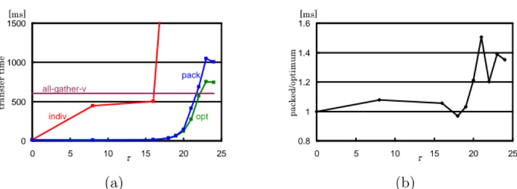
(9) Vol.2010-HPC-124 No.9 2010/2/22 IPSJ SIG Technical Report 7. 7. 6. 6. 5. columns of ji,1 = i, ji,2 = i ⊕ 1, ji,3 = i ⊖ 1, ji,4 = i ⊕ 256, ji,5 ⊖ 256, ji,6 = i ⊕ 2562 and ji,7 = i ⊖ 2562 where x ⊕ y = ((x + y − 1) mod 2563 ) + 1 and x ⊖ y = ((x − y − 1) mod 2563 ) + 1. To have matrices having some random sparseness, we transformed the base matrix A by shifting its non-diagonal elements using normal random numbers with mean 0 and a certain variance σ 2 . That is, we have a matrix A(τ ) whose i-th row has seven non-zero entries at ji,1 and ji,k ⊕ x6(i−1)+(k−1) for k > 1 where xl is the l-th element in a random number sequence x1 , . . . , x6·2563 with σ = 2τ ⋆1 . A generated matrix of 2563 × 2563 or 224 × 224 is then split into 64 submatrices of equal size, 218 rows for each, to assign each of them to each process. Therefore, the vector v is 224 -dimensional while each subvector v p is 218 -dimensional. Finally, in order to compensate excessive randomness and sparseness of the matrix resulting in a unrealistically large number of fragments in Vpq for a process pair p and q due to our straightforward generation with random shifting, we reduce the number of fragments to 210 by filling small size gaps with virtual components. We measured the time of vector transfer varying σ from 0 for A to 224 for A(24) which are almost uniformly random sparse. For each matrix, the times with the individual and packed method are also measured together with the optimum method. In addition, we measured the time of MPI_Allgatherv(), which is independent from σ, to give the whole of vector v to all processes. Fig. 4 shows measured transfer times in (a) and the ratio of those of the packing method over the optimum method in (b). Note that τ = 0 in Fig. 4(a) does not mean σ = 20 = 1 but means σ = 0. The graphs exhibit that the packing and optimum methods work well taking about 10 ms or less and almost tie for τ ≤ 16, which means vector components in a subvector v p are required only by two adjacent processes p ± 1 almost always. In this range, they are much faster than the individual method, which is also faster than all-gather. Then the transfer times of the optimum and packing methods start growing but still tie until τ = 19 at which about 10 processes needs the components in a subvector, while that of the individual method steeply grows due to a flood of small size messages. After that the optimum method clearly shows its advantage. 5. indiv.. 4. indiv.. 4. r. r 3. 3. pack. 2. pack. 2. 1. 1. comb.. 0. comb.. 0 5. 10. log2 s. 15. 20. 5. 10. (a) g = s − 5. log2 s. 15. 20. (b) g = s − 2. 7. 7. 6. 6 5. 5. indiv.. indiv.. 4. 4. r. r 3. 3. pack. 2 1. comb.. 2. comb.. pack. 1 0. 0 5. 10. log2 s. (c) g = s. 15. 20. 5. 10. log2 s. 15. 20. (d) g = s + 1. Fig. 3 Costs of Simple Methods Relative to Optimum Method.. methods but also successfully finds optimum assortment of these three methods even with merely ten fragments. For example, in a case of s = g = 13, the optimum method finds three chunks of 4, 3 and 3 fragments to achieve about 10 % cost reduction from the best of three simple methods. 4.3 Vector Transfer Performance The next experiment is to evaluate the real performance of vector transfers for large scale matrix-vector multiplications. We used 64 CPU cores equipped in four nodes of HX600 to allocate 64 MPI processes of a multi-processed matrix-vector multiplication. Matrices are artificially generated using a base matrix derived from a difference equations using 7-point stencil for a 3-dimensional 2563 grid space with periodic boundary. Since the base matrix A is constructed by a lexicographical ordering on grid coordinates, the i − th row of the matrix has non-zero entries in its. ⋆1 Therefore, the matrix is meaningless in the sense of mathematics nor physics.. 5. c 2010 Information Processing Society of Japan ⃝.

(10) Vol.2010-HPC-124 No.9 2010/2/22 IPSJ SIG Technical Report. some heuristics to reduce O(m3 ) time complexity in a practical sense; use more accurate cost functions to incorporate the effect of process mapping, memory layout of fragments, and so on; improve the communication scheduling especially when communication pattern is (almost) all-to-all. Acknowledgments A part of this research work is pursued as a Grantin-Aid Scientific Research #20300011 and #21013025 supported by the MEXT Japan.. [ms] 1.6 packed/optimum. transfer time. [ms] 1500. 1000. pack all-gather-v 500. indiv.. opt. 0. 1.4 1.2 1 0.8. 0. 5. 10. (a). τ. 15. 20. 25. 0. 5. 10. τ 15. 20. 25. References. (b). 1) Konishi, M., Nakada, T., Tsumura, T., Nakashima, H. and Takada, H.: An Efficient Analysis of Worst Case Flush Timings for Branch Predictors, IPSJ Trans. Advanced Computing Systems, Vol.48, No.SIG8 (ACS18), pp.127–140 (2007). 2) Nakashima, H.: T2K Open Supercomputer: Inter-University and Inter-Disciplinary Collaboration on the New Generation Supercomputer, Intl. Conf. Informatics Education and Research for Knowledge-Circulating Society, pp.137–142 (2008).. Fig. 4 Vector Transfer Time (a) and Comparison of Optimum and Packing Methods (b).. over the packing with 20–50 % performance superiority. However, their advantage over all-gather disappears when τ is large to make it necessary for a process to gather fragments from all other processes, due to our simple communication scheduling with a batch of non-blocking receives followed by a series of nonblocking (for optimum) or blocking (for packing) sends. 5. Conclusion In this paper, we discussed an efficient algorithm to exchange fragments of a block-decomposed vector among processes for iterative sparse matrix-vector multiplication with a matrix also block-decomposed. For a process pair p and q and the transfer of the fragments in the subvector residing in q and required by p for its local multiplication, our algorithm analyze p’s submatrix to find the optimum assortment of the fragments for individual, packing or combining transfer of them using dynamic programming technique. We implemented the algorithm on our T2K Open Supercomputer and measured its performance using 64 CPU cores to which 64 MPI processes are allocated. The evaluation with artificially generated matrices of 224 × 224 confirms our optimum method is much faster than all-gather type method when the fragments are not widely distributed among processes, and outperforms the packing method especially when the size of gaps between fragments varies widely. Our urgent future work is to evaluate our method with realistic matrices. We also plan to improve the performance of our method by the followings; introduce. 6. c 2010 Information Processing Society of Japan ⃝.

(11)