Journal of the Operations Research Society of Japan
Vol. 27, No. 2, June 1984
A
NONSMOOTH OPTIMIZATION APPROACH TO NONLINEAR
MULTICOMMODITY NETWORK FLOW PROBLEMS
Masao Fukushirna Kyoto University
(Received September 2,1983: Revised February 10,1984)
Abstract This paper is concerned with the convex cost multicommodity flow problem. First, it is shown that the Lagrangian dual of the problem can be formulated as a convex nonsmooth optimization problem. Then, an algorithm is presented for solving a problem which is obtained by slightly modifying the dual problem so as to be amenable to shortest chain algorithms. Since the proposed .!lgorithm mainly consists of successively solving shortest chain problems and linearly constrained subproblems whose size is independent of the underlying network structure, we may expect that it can solve fairly large problems. Convergence of the algorithm is proved and several remarks on its implementation are given. Finally, limited computational experience with the proposed algorithm is reported.
1. Introduction
One of the most important network optimization problems is the class of multicommod:i.ty flow problems [1,18]. The multicommodity network flow problems may be classified into two categories, linear and nonlinear models, according to a type of the cost function to be optimized. The nonlinear models have, in particular, been extensively studied in connection with design and analysis of urban traffic systems and communication systems. Typically, the equilibrium traffic assignment problem in a transportation network [2,6,20] and the optimal routing problem in a packet switched com-puter network [5,10,14] lead to convex cost multicommodity flow problems. In those problems, the nonlinear dependence of costs on the flow is intrin·-sic because of congestion effects in the network.
In this paper, we present a new approach to the solution of convex cost multicommodity flow problems. We first show that the dual of the multicom·-modity flow problem can be formulated as a problem of maximizing a concave objective function subject to simple bounds on the variables. We also
152 M. Fukushima
point out that the dual objective function is nondifferentiable but its functional values and subgradients can conveniently be calculated by using an efficient shortest chain algorithm. We then develop a nonsmooth opti-mization algorithm of deseent type for solving the dual problem. The algo-rithm is a modified and extended verSion of the one presented in [11], which takes special features of the problem into account. Once the dual problem is solved, it is straightforward to recover an optimal solution of the original multicommodity flow problem.
Our approach may thus be considered an adaptation of a nonsmooth opti-mization technique to the dual method for the non linear multicommodity flow problems and is significantly different from those which are available for problems of similar nature. Indeed, the majority of existing algorithms such as [3,8,13,20] fall into the category of feasible direction methods for linearly constrained optimization. Duality results concerning the traffic assignment problems may be found in [12,15J, but it appears that only a few attempts have been made to solve those problems from a dual or primal-dual point of view [23,26]. On the other hand, the column generation technique, which is essentially a dual method, has been adapted to solve a variety of linear cost multicommodity flow problems [9,29]. It is also noted that the subgradient algorithm, which is a popular heuristic nonsmooth optimization technique, has been successfully applied in the context of the primal decom-position approach to the linear multicommodity flow problems [16,19].
This paper is organized as follows: In the next section, we explicitly formulate the convex cost multicommodity flow problem. In Section 3, we derive the dual problem and show that an optimal solution of the multicom-modity flow problem can be obtained by solving it. In Sections 4 and 5, we describe an algorithm for solving the dual problem, prove its convergence, and make some comments on the implementatio~ of the algorithm. In Section 6, we present results of numerical experiments to demonstrate the effectiveness of the proposed algorithm.
2.
The Nonlinear Multicommodity Flow Problem
Consider a directed network with a finite set N of nodes and a finite set A of arcs. Let K denote the set of commodities to be transported through the network. We suppose without loss of generality that each com-modity has a single origin-destination (O-D) pair which is different from those of other commodities.
(1)
where
Nonlinear Multicommodity Flow Problems
The minimum cost multicommodity flow problem may be formulated as min
L
f (L
xk) aEA a kEK a s. t. k kL
x aEOU)aL
x aEIU)a k :?: 0 x a{
-DDk k 0 'ila c A,
'ilk E K kx flow of commodity k on arc a a
i f i=s k i f i = tk otherwise
,
Dk known nonnegative flow requirement for commodity k (sk,tk): O-D pair for commodity k
O(i) set of arcs originating at node i IU) set of arcs terminating at node i f cost function for arc a.
a
In words, the problem is to minimize thE! sum of arc costs which are func-tions of total arc flows
x a k x a 153
subject to the flow conservation equations and the nonnegativity constraints. The arc cost functions f
a are supposed to be nonlinear in order to take into account congestion effects in the network. Many authors assume f is everywhere finite--valued but f (x) increases
radi-a a a
each function
cally as xa exceeds a substantial capacity of that arc, thereby forcing the solution of problem (1) to meet capacity requirements. This trick may sometimes be helpful, because then the problem turns out to be formally un-capacitated. In this paper, however, we allow the possibility of including arc capacities explicitly by assigning the value -too to f (x )
a a for x a greater than the capacity of arc a . It will be seen that such an extension does not cause any difficulty in dealing with problem (1) by way of its dual problem.
In the sequel, we assume the follmling: closed convex function with effective domain
For each dom f a EA, fa is a f (x ) < -too a a { x a being an interval such that [O,ca )
infinite) positive capacity of arc and nondecreasing on dom f
,
anda or [O,c a
1
,
a Moreover, lim f (t)/t t->-too a a where f a c a is a (possibly is strictly convex -too whenever c=
-too •154 f (x ) a a D = [O,e ) a a Figure 1. M, Fukushima f (x ) a a
Arc cost functions f
a
f (x )
a a
(c) e = -+<>0 , D
=
[0,-+<>0)a a
These assumptions are natural enough to meet desirable properties of the cost functions. Typical examples of fa are illustrated in Figure 1.
The minimum cost mu1ticommodity flow problem can alternatively be stated in terms of flows through chains of the network. To be specific, let P
k denote the set of a11,chains of arcs between O-D pair (sk,tk) for commodity k . Since O-D pairs are distinct for all commodities, we have
P
k n Pk, = I/J i f k '" k' Let us denote by Yp the flow through chain p x and the chain flows Y can be related by
a p
(2) x
a <5 ap p Y Va E A ,
Then the total arc flows
where <5 are elements of the arc-chain incidence matrix of the network, ap
i.e. ,
if arc a is on chain p otherwise.
The arc-chain formulation of the minimum cost mu1ticommodity flow problem is now given by
(3) min
I
aEA s. t.Nonlinear Multicommodity Flow Problems
f ( I
Icy)
a ap p kEK PEPk Y ~ 0 , p 155The above formulation presupposes that we have an enumeration of chains for each O-D pair (sk,tk) This appears to be unrealistic for networks one encountered in practice. In the development to follow, however, we shall be concerned with the arc-chain formulation (3) rather than the node-arc formulation (1). This is simply for convenience of exposition and, in fact, the algorithm proposed later will not require such chain enumeration.
3. Dual Problem and Its Properties
In this section, we develop duality theory for the mu1ticommodity flow problem as formulated by (3). In what follows, we shall make extensive use of results from convex analysis [27]. In particular, for an arbitrary convex function f , we denote by f* the convex conjugate function of f , i.e.,
f* (u)
=
sup { u x T -f(x) },
'ilu xAlso, we denote by Clf(x) the set of subgradients of f at x , i.e. ,
Clf(x)
=
{ u f(x' ) ~ f(x)+
u T (x' - x),
'ilx' }Using the relation (2), we may rewrite problem (3) as the following linearly constrained convex programming problem
(4) min
I
f (x ) aEA a a s.t. xI I
<5 apYp 'iI a E A a kEK PEP kI
Y = Dk ' 'ilk E K PEP k p' Yp ~ 0 'ilp E Pk ' 'ilk E K •The Lagrangian for problem (4) is then defined to be
L(x,y,u,v)
I
f (x ) -I
u { xI I
<5 apYp }a a a a
aEA aEA kEK PEP
156 M. Fukushima
L
Yp - Dk } , PEPk where u
a and are Lagrange multipliers (dual variables), and x, Y , u and
(5)
v are the vectors with elements xa' Y
k ' ua and vk ' respectively. Now we may state the Lagrangian dual tu problem (4) as
max 2(u,v) ,
where the dual objective function 2 is given by (6) 2(u,v) inf {L(x,y,u,v)
I
Y ~ 0 }X,Y inf
L
x aEA [ (x ) - u x } a a a a+
infL L
L
u0
-
vk } Yp aEA a ap Y~O kEK PEPk
=
aEA a a kEK k k1
-
L
f* (u )+
L
D v i fL
u 0 ~ V k ' V P E Pk , V k E K aEA a ap - 0 0 otherwiseIn view of (6), problem (5) is explicitly represented as
(7) max
L
f* (u )+
L
DkV k a a aEA kEK s. t.2:
u0
~ Vk ' V P E P k V k E K . aEA a apNoting that Dk are all nonnegative, we may further rewrite problem (7) as
(8) max f*(u )
+
a a u a ap
0
Since the conjugates f~ are closed convex functions and the second term of (8) is piecewise concave in u , (8) is a problem of maximizing a concave function which involves only the variables
It is important to note that each f* a
u a
is a function of a single vari-able u
a This fact enables us to obtain an explicit representation of f* a in most application situations. Furthermore, as a consequence of the assump-tions on f , the functions f* enjoy quite favorable properties as shown
a a
Nonlinear MUlticommodity Flow Problems 157
Proposition
1. For each a EA, the function f*a is everywhere finite and continuously differentiable.
Proof:
The assumptions on f imply that each f is co-finite [27,a a
p.116]. It 'then follows from [27,Cor.13.3.1] that the conjugate everywhere finite-valued. The continuous differentiabi1ity of from [27,Thm.26.3 and Cor.25.5.1].
D
f*
a
f* is a
follows
Now let us turn our attention to the second term of the objective func-tion of problem (8). By inspection, it is easy to see that the minimization problem (9) min PEP k
L
aEA U <5 a apis nothing but a problem of finding the shortest chain between O-D pair k k
(s , t ) in the network with arc lengths given by u
a ' a EA. We may
therefore use an efficient shortest chain (path) algorithm [7] to evaluate (9). However, since the shortest chain algorithm generally requires arc lengths to be nonnegative, it will be convenient to make a slight modifica-tion of problem (8).
Let et
a denote the right derivative of
et a 1im t+O f (t) - f (0) a a t f a at x a Since f
a is assumed to be convex and nondecreasing on and is nonnegative for every a EA.
(10)
We consider the problem
max
L
aEA s. t. f*(u )+
a a u 2': et , minL
PEP k aEA u a ap0
o ,
Le., dom f a et a existswhere et is the vector with elements a'a' a EA. The only difference be-tween problems (8) and (10) consists in the existence of the simple bounds on u
a in the latter problem. It is to be noted that the shortest chain problem (9) does not contain any arc with negative length, provided u is feasible to problem (10).
The next proposition assures that problem (8) can be replaced by problem (10) without loss of generality.
Proposition 2.
(i) The optimal values of problems(8)
and (10) are equal. (ii) Any optimal solution of problem (10) also solves problem (8).158 M. Fukushima
(iii) If problem (8) has an optimal solution, then problem (10) also has an optimal solution.
Proof:
Under our assumptions on(11) f* ( U )
= -
f (0)a a a
f , it can be shown that a
for any u $ Cl.
a a
To prove (i), suppose. there exists a point
'il
such that the correspond-ing objective value is strictly greater than the maximum value of problem (10). Then, it is clear thatu
violates the constraints u ~ Cl. of problem (10).Let
u'
be defined byr
i f ~, u a u ~ Cl. (12) u=
a a a i f < Cl. Cl. u a a aObviously,
il'
is feasible to problem (10). Moreover, the objective value at'il'
is 10 less than that atu,
because of (10) and the fact that the second term of the objective function is nondecreasing with respect to 'U • This is a contradiction and proves (i).Since problem (8) is a relaxation of problem (10), (ii) follows trivially from (i). To see (iii) holds, it suffices to note that, if u is an optimal solution of problem (8), then the point
'il'
constructed by (12) turns out to be optimal to problem (10). 0In order to validate our dual approach to the multicommodity flow prob-lem, it remains to show that the optimal solution of problem (4) can actually be obtained by solving problem (10). The following proposition asserts this.
Proposition 3.
Suppose problem (4) has a feasible solution such thatX E int dom f a a of the interval for all dom f a
a EA, where int dom fa stands for the interior Then, both problems (4) and (10) have optimal solutions and the optimal values of the two problems are equal to each other. Furthermore, if u solves problem (10), then the point x uniquely deter-mined by the formula
(13) x a V'f*("U ) ,
a a a E A
constitutes a part of an optimal solution of problem (4).
Proof:
Consider problem (4) and its dual (7). Clearly, problem (4) has an optimal solution, say(x,y)
Then, the hypothesis of the proposition guarantees [27,Cor.29.l.4] that there exists a vector ("U,;) satisfying the following Kuhn-Tucker conditions [27,Thm.28.3] for problem (4):U
E df(x ) ,
Nonlinear Multicommodity Flow Problems 159
L L
<5 -x apYp .a kEK PEP k 'r/ a E AL
Yp = Dk ' PEP k 'r/ k E KI
u <5 ~ Vk ' Yp ~ 01
aEA a ap Yp > 0 ==0>I
u <5 Vk aEA a apTherefore, it follows from [27,Thms.30.3-5] that (~,;) solves the dual problem (7) and the optimal values of problems (4) and (7) are equal. More-over, since f* a is differentiable by Proposition 1 and Vf* is the inverse
a mapping of
relation in
df
a [27,Cor.23.5.l], the formula (13) follows from the first the above Kuhn-Tucker conditions.
To complete the proof, it simply suffices to recall that problem (7) is a restatement of problem (8) and problem (8) is essentially equivalent to problem (10) by Proposition 2.
0
To conclude this section, we shall briefly mention an economic inter-pretation of the dual variables u and v To be specific, let us suppose that problem (4) represents an equilibrium (user-optimization) traffic assignment problem (see, e.g., [6]). Then, i t is easy to see that the Kuhn-Tucker conditions appearing in the proof of Proposition 3 are nothing but a restatement of the Wardrop's principle [30] saying that the travel times on all the routes actually used are equal and no greater than those which would be experienced by a single vehicle on any unused route. In this context, it is quite reasonable to regard u
a and a and the minimum travel time between O-D pair
as the travel time along arc k k
(5 ,t ) , respectively (see the first and the last relations in the Kuhn-Tucker conditions). Therefore, the dual problem (7),(8) or (10) may be considered an alternative formula-tion of the traffic assignment problem, in which the variables are travel times, rather than traffic flows, in th!~ transportation network.
4.
Algorithm for Solving the Dual Problem
As shown in the previous section, the dual of the multicommodity flow problem can be formulated as problem (10) which involves a concave but non-differentiable objective function. We might therefore apply any of the existing general-purpose algorithms for nonsmooth optimization [22,25] to
160 M. Fukushima
solve problem (10). In this and the next sections, however, we shall develop a specialized algorithm for solving problem (10). The proposed algorithm is an extension of the nonsmooth optimization method presented in [11] and is designed to take special features of problem (10) into account. In particu-lar, i t may take advantage of second order information on the objective function, and hence is expected to work more efficiently than those which exploit only subgradients of the objective function.
In the development to follow, we shall be concerned with the problem equivalent to (10):
(14) min F(u)
s. t. u 2: Cl. ,
where F is a convex function defined by (15) F(u) =
I
aEA
f*(u )
a a u a <5 ap
In this section, we present a basic framework of the algorithm for solving problem (14) and prove its convergence. Subsequently, in the next section, we shall discuss the implementation of the algorithm in some detail.
The algorithm is doubly iterative in itself and starts with a point ul arbitrarily chosen from the feasible region of problem (14), i.e., ul 2: Cl. •
Let E,
S
and m be prescribed real parameters such that E > 0 , 0 <S
< 1 and 0 < m < 1that (16)
k
Generally, on the kth major iteration, we are given a point u such
k
u 2: Cl. and try to obtain an approximate solution of the problem min
s. t. z 2: Cl. ,
where cfJ
k is a function defined by
(17)
and Bk is a positive definite matrix. Problem (16) is again a nonsmooth optimization problem, but involves a strongly convex objective function.
It is noted that, if Bk is chosen as the identity matrix I for each k , problem (16) reduces to the subproblem of the proximal point al-gorithm [28] and its solution provides the minimum norm E-subgradient (27, p.2l9] for some E >
o.
(See [11] for detailed arguments.) Here we do not restrict ourselves to the special case Bk :: I , in order to better incor-porate the second order information of the objective function.
Nonlinear Multicommodity Flow Problems 161
We now c.onsider applying a cutting plane type procedure to problem (16). More specifically, we successively find an optimal solution
lowing quadratic programming subproblem (18) min z(z-u ) 1 k T Bk(Z-U ) k + n
i
z to the
fol-s. t. F(zj)
+
(~)T(z_zj) ~n ,
j 0,1, ... ,i-lz
~a ,
where z
o
is a subgradient of F at We shall callthis process the inner iteration.
Let 1jJk . ,~ denote the optimal value of problem (18). Since are subgradien ts of F at zj , it is not difficult to see that
~k
.,~ always
affords a lower bound of the optimal value of problem (16). Moreover, as will be shown shortly (Proposition 4), 'Ne must eventually have either
(19)
~k
.+
E,~
or
(20)
S {
F(u ) -k 1jJk .-,~
for some i ,where E and
S
are the parameters specified previously. The conditions (19) and (20) serve as stopping criteria for the major and inner iterations, respectively.Therefore, for each i , we first eheck the condition (19). I f (19) is satisfied, we terminate the major iteration itself. When (19) is not met, we next check the condition (20). If (20) also fails to hold, we continue the inner iteration with i increased by one. On the other hand, i f (20) is achieved, we define a search direction by
j { i k d - = z - u
and then determine a step length tk ~ 1 satisfying (21) and (22) where (23)
Uk+tkjc~a,
is given by 1 k T*
o = -(l-S)E - -(d) B o-k 2 k162 M. Fukushima
k+l k Jc
u ,. u
+
ta-k
and proceed to the next major iteration with k increased by one. It is to k
be noted that the sequence {u} thus generated lies in the feasible region of problem (14) and {F(Uk)} is a monotonically decreasing sequence.
The above procedure is summarized as follows: Step 1: Choose u 1 ~ Cl. and set k = 1
.
2: Select 0 k 0 0
Step Bk put z
=
u,
choose g E: (IF(Z ) and set i 1 Step 3: Solve (18) to obtain Z i and~k
.,~
Step 4: I f (19) is satisfied, terminate. Otherwise, go to Step 5. Step 5: I f (20) is satisfied, then set et= Z i - u k and go to Step 6.
Otherwise, choose g i E: (IF(zi)
,
set i=i+l and return to Step 3.Step 6: Determine tk ~ 1 satisfying (21) and (22) • Set u k+1 uk
+
tket and k = k+
1 , and return to Step 2.The next two propositions demonstrate that each step of this algorithm is always consistent.
Proposition 4.
At each major iteration k , either (19) or (20) issat-isfied for some i .
Proof:
Suppose to the contrary that, for some k , neither (19) nor(20) is achieved for each i Then, we must have
and for all i (24) for all i where <P* k >
S
{F(U ) k -lJl -k ,~ .}Combining these inequalities, we get
i
-<Pk(z ) - lJlk,i > SE
However, it can be shown in a way similar to [11,Prop.3] that
~im
<Pk(zi)=
1im~k
.=
<Pk '~-- i--'~
is the optimal value of problem (16), which is finite by the strong convexity of <P
k • This contradicts (24) and the proof is complete.
0
Proposition 5.
Suppose that, at major iteration k ,(19)
fails to holdbut (20) is satisfied for some z i satisfying (21) and (22) is nonempty.
Then, the set of step lengths
Proof:
I t suffices to show that the step length of unity, tk=
1,sat-k Jc .
con-Nonlinear Multicommodity Flow Problems
struction of Z i ,we only prove that (21) is satisfied by
hypotheses, we have
and
4>k(Zi) $ 13F(uk)
+
(l-13)~jk,i
These inequalities together with (17) imply
tk
=
1. By ouri k 1 i k T i k
F(z) < F(u ) - (1-13)£ - i(z -u ) Bk(Z -u ) •
Noting that zi. = uk
+
if ,
we obtain from the last inequality and (23)k J( k
F(u
+
(r) < F(u )+
OkThis implies that (21) is fulfilled by
tk
= 1 ,because 0 < m < 1 and Ok < O.0
163
The proof of the last proposition suggests that we may simply set tk
=
1 for all k . From the viewpoint of computational efficiency, however, it is tempting to obtain more satisfactory improvement in the objective value at each iteration by allowing tk to be greater than unity. We shall provide a simple line search procedure suitable for the present problem in the next: section.Now we consider the convergence properties of the proposed algorithm. The following proposition states that the algorithm always terminates after generating a point which can be regarded .as an approximate optimal solution
to problem (14), whenever certain boundedness conditions are met.
Proposition 6.
Suppose that the fun(:tion F is bounded from below andthe positive definite matrices Bk are uniformly bounded, Le., there exists a A > 0 such that
(25)
Then, the algorithm terminates in a finitt~ number of iterations and the last iterate uk satisfies the following approximate optima1ity condition
(26) Vu •
Proof:
Suppose that the algorithm lasts infinitely, i.e., the condition(19) is never achieved for any k and i . Then, since the inner iteration terminates finitely for each
{uk} h
sequence Noting t at
we obtain from (21) and (23)
k by Proposition 4, we must have an infinite Bk are positive definite and tk 2 1 , however,
164 M. Fukushima
which in turn yields
F(uk+1)
~
F(Ul) - kmdl-(3)''ilk •
This implies F(uk) tends to _00 as k
~
00 and contradicts the assumption that F is bounded from below. Thus the algorithm must terminate finitely.k
Now let u be the last iterate generated by the algorithm. Define the function W k by A k 2 W k (z)
"2
11 z - u 11+
F(z).
Obviously, we have (27) W k (u k ) F(u ) k and, by (25), (28) <Pk(z) ~ W k (z) 't:/z • Moreover, since we have~k
,~ . is a lower bound of the optimal value of problem (16),(29) 't:/z •
It then follows from (27),(28),(29) and (19) that
(30) 't:/z •
Using the notion of E-subdifferential [27, p. 219], we have an equivalent representation of (30) (31) is the E-subdifferential of
W
k
at k u , i.e., k T k Wk(u) ~ W k (u )+
~ (u - u ) - E, 't:/u }Furthermore, applying a formula for the E-subdifferential of the sum of con-vex functions [17,Thm.2.l1 to the function
W
k , we have (32) dEWk(uk) c
12AE
B+
dEF(Uk) ,where B is the closed unit sphere. Combining (31) and (32), we may con-clude that there exists a
~
EO dEF(Uk) such thatII~II
5 IZAE Consequently, by the definition of E-subdifferential, we obtain for any uF(u)
~
F(uk)+
~T(u
- uk) - ENonlinear Multicommodity Flow Problems
o
Note that the boundedness assumption on F is satisfied under the hypothesis of Proposition 3, which is normally fulfilled in practice. Also we mention that the approximate optimality condition (26) has been consid-ered in [11,21].
165
To conclude this section, we should mention that the number of inner iterations required to achieve (20) usually increases as the major iteration proceeds. Unfortunately, we have been unable to establish any theoretical bound on the number of inner iterations with E, Sand k given. In our preliminary computational experiments reported in Section 6, however, the condition (20) was always attained before subproblem (18) became intractably large.
5.
Remarks on the Algorithm
In this section, we provide some guidelines concerning the implementa--tion of the proposed algorithm.
5.1. Eval uation of subgradients of F
In order to construct subproblems (18), it is required to supply a sub-routine that calculates, for any feasible point of problem (14), a subgradient of the function F defined by (15). It is noted that the functions f* are
a
continuously differentiable (Proposition 1) and their gradients are in gen-eral available explicitly. Therefore, it would be sufficient to show how we can obtain a subgradient of the concave function h defined by
min
I
PEP k aEA
u
0
a apAs was pointed out in Section 3, h(u) can be evaluated at each u by solving the shortest chain problem (9) for each k E K. Note that the arc lengths u
a are all nonnegative, because we are exclusively concerned with feasible points of problem (14). Denote
P (u)
k U a
0
ap U a0
aqi.e., Pk(u) is the set of all shortest chains for commodity k when arc lengths are given by u
a ' a EA. Then, it can be shown [12] that, for any Pk E Pk(u) , the vector with elements
166 M Fukushima
I
a E AkEK
affords a subgradient of h at u Thus, a subgradient of h can be readily obtained as a byproduct of evaluating the functional value of h
Consequently, a subgradient of the function F at u is given as the vector whose elements are
Vf*(u ) -a a
5.2. Choice of matrices Bk
I
a EA,kEK
In view of problem (18), it seems quite reasonable to choose matrices
Bk so as to take account of second order information on F Since the second term of (15) is piece-wise linear in u, we confine ourselves to information obtained from the first term
f* a is continuously differentiable at any
L
f*(u ) . By proposition 1, each a au
a Moreover, it happens in most applications that t* actually has the second derivatives.
a
Assume the existence of V2f*(u) for each u Then we may consider
a a a
as a diagonal matrix with diagonal elements it appropriate to define Bk
V2f*(uk) . (If V2f*(U) does not exists or is difficult to calculate
ex-a a a a
p1icit1y, we may replace it by from the first derivatives of
a finite difference approximation obtained
f*.) Note that V2f*(uk) is never negative
a a a
thanks to the convexity of
f:
However, since it may happen that V2f* a take value zero or be~ome unbounded, it is necessary to modify the defini-tion of Bk as(33) Bk
where bk are given a (34) bk a
=
diag(bk) a,
by.
{
m a V2f*(uk) a a M a i f i f i f "if*(uk) < m a a a m ,,; ,if*(uk) a a a V2f*(uk) > M a a a ,,; M afor some 0 < m < M By this modification, the matrices Bk are assured a a
to be bounded and positive definite, and hence the hypothesis of Proposition 6 is fulfilled.
Nonlinear Multicommodity Flow Problems 167
5.3. Solving subproblems (18)
At each major iteration. we are required to solve a sequence of convex quadratic programming problems
(18).
Although those problems may be treated in a direct manner by any quadratic programming algorithm. we consider it more effective to transform problems(18)
into problems of smaller size by means of a variable reduction technique and then solve the latter problems using a suitable optimization algorithm. It will become evident that this idea is remarkably useful when the network under consideration is large. In the development to follow. we suppose that Bk is a diagonal matrix as given by (33) and (34).(35)
To simplify the notation, let us rewrite problem
(18)
as min s. t.t(Z -
uk) TBk(Z - uk)+
n
T G Z - ne :s; q Z ;?: a. •where G
=
(g ••••• go
i - l O T ) . q=
«g ) Z 0 - F(z ) ••••• 0 (g i-I T i-I ) Z - F(z i-I T»
and e=
(1 •...• 1) T Then. the Lagrangian associated with problem (35) is defined to be1 k T k T T T
8(z,n,ll,V) = 2(z-u) Bk(Z-U)
+
n+
II (G z-ne-q)+
v
(o.-z) , where II andv
are the vectors of Lagrange multipliers. Since Bk is positive definite, problem (35) has a dual which is given by direct calcu-lation as (36) max s.t. 8(ll,V) T e II=
1 •where 8 is a concave quadratic function defined by
(37) 8 (ll. v) = v T (a. - u ) k
+
II (G T T k I T u - q) - 2(v - Gll) Bk -1 (v-Gll)Moreover, it :is not difficult to observE~ that. if (ll, v) solves problem (36), then the point z given by
(38) z
=
u k+
Bk -1 (v - Gll)constitutes an optimal solution of problem (35).
The quadratic programming problem (36) can be solved in two stages: We first maximize 8(1l,V) with respect to \I for fixed ll, and then maximize
h 1 · f ti . h t t As B
k
-l is also positive t e resu t1ng unc on W1t re spec 0 ll.
168 M. Fukushima
definite and diagonal, the first stage of the above procedure can easily be carried out and yields
(39) v(~) max { 0 , G~ -Bk (u -k et) }
as the maximizer of e(~,v) with respect to V Substituting (39) into (37), we may explicitly state the second stage problem as
(40) max s. t. '¥ (~) T e ~
=
1 , where f is defined by T T k ~ (G 11 - q)In addition, it can be sho~m that '¥ is a concave function and has a con-tinuous first derivative explicitly given by
T k T -1
'V'¥(~) = G u - q - G Bk (~-v(~»
Thus, problem (40) is a differentiable concave programming problem with a single equality constraint and the nonnegativity constraints.
It should be noted that the number of variables in problem (40) is just equal to the iteration COllilt of the inner iteration. More important is the fact that the size of problem (40) is, unlike problems (35) and (36), free from the size of the underlying network. Therefore, the variable reduction process described above will be considerably meritorious when we are in-· volved in large networks.
One thing which might obstruct the present approach is the fact that problem (40) is not a quadratic programming problem any more and hence we cannot expect to obtain its exact solution finitely. Our computational experience reveals, however, that a good approximate solution to problem (40) can be obtained quite easily and such approximation does not cause breakdown of the algorithm, provided a proper approximation criterion is used.
5.4. Line search
Although the step size of unity is sufficient for convergence of the algorithm as pointed out just after the proof of Proposition 5, looking for a step length t 2 1
k seems worth considering since it would afford a more
satisfactory decrease in the objective value. However, since evaluating
F(u) amounts to solving shortest chain problems (9) for all commodities,
Nonlinear Multicommodity Flow Problems
are not recommlmded. Bearing this in mind, we present a very simple line search procedure which appears to be suitable for our problem.
169
Recall that the directional derivative of the convex function F at u with respect to a direction d may be characterized by
T
F' (u;d) = sup {g dig E dF(u) }
[27,Thm.23.4]. Therefore, for any g E: cIF(u) , the quantity Y = gTd affords a lower bound of F'(U;d) and, i.n particular, it coincides with F' (u;d) whenever F is differentiable at u .
Given the current estimate uk of the optimal solution and the search direction
~,
the line search algorithm proceeds as follows: First we take t = 1 and calculate y = gT? for an arbitrary g E:dF(uk+~)
•1 If Y
l ?: 0 , then we set because Y
l ?: 0 implies
tk
=
1 and terminate the line search procedure, F(uk+ t~)
is nondecreasing for t > 1 . IfY
l < 0 , then we calculate the maximum step length condition (22), i.e., Note that t max t max ?: 1 by the construction of t
max satisfying the
There are two possibilities for the values of t
max That is, (i) t: max < +00 and (ii) t max Tk
In case (i), we calculate
Y
2
=
ga
for an arbitraryY
2
~
0 , we may conclude that F(u k+
tdk) is mono tonically g E: dF(uk+t,I)
max I f in the interval [1, t ] . max fies condition (21), and setTherefore, \.re set tk
=
1 otherwise. normally met by tmax as long as the parameter On the other hand, when Y
2 > 0 , a minimizer of
nonincreasing
t
=
t if tsatis-k max max
Note that condition (21) is rn is set sufficiently small.
F(uk
+ t~)
lies in the interval [l,t ] . We may obtain an approximate minimizer, sayt ,
bymax
carrying out a single step of the cubic interpolation [24,p.142] using the functional values
F(uk+~),
F(uk+ tcf)
and the (approximate) directionalmax derivatives Y
l , Y2 at t
=
1 and t=
tmax ,respectively. We then set tk=
t ift
satisfies condition (21), and set tk=
1 otherwise. Again, we usually have t=
t ,
since condition (21) is not very restrictive fork such t in practice. In case (ii), we
Y
=
gT~
,where g c those at t=
1 , we select some k k E: dF(u+ t
d ) c tc > 1. and calculate F(u
k
+
t~)
c and Based upon these values together with carry out a single step of the cubic interpolation to obtain an approximate minimizer t of F(uk+ t~).
Then, as in the previous case, the actual step length is determinE~d as tkon whether t satisfies condition (20) or not.
170 M. Fukushima
The above procedure can be implemented very easily and the generated step length tk obviously satisfies the line search criteria (21) and (22).
5.5. Choice of the parameters E:, (3 and m
The parameters £, (3 and m are supposed to be fixed throughout the iterations, though it is possible to modify the algorithm in such a way that those parameters vary on every iteration without impairing the convergence properties.
As shown by (26), £ is a tolerance parameter which indicates how close
the approximate solution u k obtained by the algorithm is to the true opti-mum. So, £ should be set small enough to meet the user's requirement on
the accuracy of the approximate solution.
The parameter (3 used in the termination criterion of the inner itera-tions seems to have the greatest influence on the performance of the algo-rithm. In view of (20), it is clear that assigning a large value to 13 results in a small number of inner iterations. Therefore, it is recommended to set (3 sufficiently close to one, say (3
=
0.99999 , because spending too much time in the inner iterations is obviously undesirable for the over-all performance of the algorithm.The parameter m appearing in the line search criterion (21) plays a relatively minor role in the algorithm. We suggest that a sufficiently small m, say m = 0.1 , may be suitable for the line search procedure descr:ibed in 5.4.
6. Computational Results
In order to measure the efficiency. of the proposed algorithm, limited computational experiments have been conducted on several traffic assignment test problems. In the traffic assignment models, the commodities correspond to prespecified O-D pairs for which nonzero trip demands exist. For example, if the transportation network has m arcs and n nodes, and there are trip demands for all O-D pairs (i,j) , i , j = 1, ...
,n,
i " j , then the problem involvesn(n-1)
commodities. Thus, the traffic assignment problem as formulated by (1) containsmn(n-1)
variables. It is noted, however, that the dual problem (10) contains m variables which, as indicated at the end of Section 3, represent travel costs through the arcs.Nonlinear Multicommodity Flow Problems
are assumed to be of the form
f (x ) a a { a x a a -t«> i f x ; : : 0 a otherwise where a
a and are given positive parameters. Obviously, the right derivative of f at x
a a
are directly calculated as
f*(u ) a a
It is easily seen that
V
2f*(u) tends to -t«> a a f* a as=
0 is aa The convex conjugate functions
if U ;:: a
a a
otherwise are twice d:lfferentiab1e for
u a '" a a
171
f* a
The computer program was coded in FORTRAN 77 and the runs were made on a FACOM M382 computer at the Data Processing Center, Kyoto University. To solve subproblems (40), we used a subroutine LCQNDR in the NPL Numerical Optimization Software Library developed by the National Physical Laboratory, England. Also, we employed the Warsha11-F1oyd algorithm [7] for finding shortest chains between all pairs of nodes to solve problems (9). The param-eters
B
and m were set at 0.99999 mld 0.1, respectively. The lower and the upper bounds on the diagonal elements of Bk (cf. (34» were specified as m=
200 and Ma a 20,000 , respectively, for all a EA.
First, we applied the algorithm to six fictitious test problems whose data D
k , aa and Ba were chosen in a random but plausible manner so as to imitate actual traffic situations. Each problem was solved with two different values of E , i.e., E
=
0.1 and E=
0.05. The size of each problem and the experimental results are summarized in Table. Table shows that the CPU times are roughly proportional to NSUB and NFUN. This is implied by the fact that most of the computational effort is devoted to solving subprob1ems (40) and shortest chain problems (9). We also mention that, as far as these numer-ical examples are concerned, we never encountered a case in which a single major iteration involved more than fifteen inner iterations. Although the number of inner iterations to be perfonned in a single major iteration was gradually increasing as the major iteration proceeded, this phenomenon will not impede the use of the algorithm unless we insist on obtaining a very accu-rate approximate optimal solution to thl~ problem.172 M. Fukushima
Table. Problem data and computational results Problem I1 nodes tI arcs I1 commodities E ITER NSUB NFUN
1 7 20 42 0.1 6 7 8 0.05 6 8 9 2 7 20 42 0.1 5 6 6 0.05 6 8 8 3 12 34 132 0.1 10 47 55 0.05 13 87 97 4 12 34 132 0.1 14 46 54 0.05 18 87 97 5 16 25 240 0.1 9 20 28 0.05 14 38 50 6 16 25 240 0.1 28 51 79 0.05 65 162 190 ITER: Number of major iterations.
NSUB: Number of subprob1ems (40) solved.
NFUN: Number of function evaluations, i.e., number of shortest chain problems (9) solved.
N.B. NSUB is equal to the total number of inner iterations.
CPU sec. 0.059 0.062 0.054 0.062 0.527 1.077 0.426 0.732 0.207 0.385 0.465 1. 339
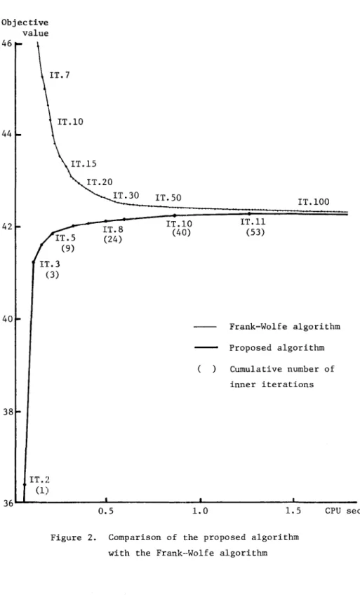
In order to examine the algorithm further, we also solved the test
t
problem given in [20]. The problem contains 24 nodes, 76 arcs and 552 commodities. The behavior of the algorithm applied to this problem is illustrated in Figure 2. I t is noted that the vertical axis in Figure 2 represents the objective value of the original dual problem (10) rather than problem (14).
{uk} ated sequence
Therefore, the objective value corresponding the gener-is m0l1otonica11y increasing. It is seen from Figure 2 that the algorithm converges very rapidly in particular at an early stage of the iterations. The same problem was solved by the Frank-Wo1fe algorithm
[20], which is known as one of the most effective methods for non1inear mu1ticommodity flow problems, and the computational result is also
illustra-ted in Figure 2. Since a single iteration of the Frank-Wo1fe algorithm consists of solving a shortest chain problem to find a search direction and performing an exact line search procedure, it is roughly comparable to a single inner iteration of the proposed algorithm. For accuracy purposes, however, the results presented in Figure 2 are based on the CPU time. We have also compared the solutions obtained after 100 iterations of the
Frank-tIn [20], the trip table is erroneously 1abe1ed as thousands of vehicles per day. The correct units are hundreds of vehicles per day.
Objective value 46 44 42 40 38 IT.3 (3) IT.2 (1)
Nonlinear Multicommodity Flow Problems
IT.8 (24) IT.50 IT.IO (40) IT. 11 (53) IT.100 Frank-Wo1fe algorithm Proposed algorithm Cumulative number of inner iterations 36~---~---~---~---0.5 1.0 1.5
Figure 2. Comparison of the proposed algorithm with the Frank--Wolfe algorithm
CPU sec. 173
174 M Fukushima
Wo1fe algorithm with those obtained after 11 major iterations of the proposed algorithm. (Note that 100 Frank-Wo1fe iterations are approximately equal in CPU time to 11 major iterations of the proposed algorithm.) In the compari-son, the solutions obtained by the proposed algorithm were transformed into flow values using the relation (13), and we found that there was no differ-ence between the two solutions within three significant figures for most of the variables. Consequently, we may conclude that the proposed algorithm performed at least as efficiently as the Frank-Wo1fe algorithm, as far as this test problem is concerned.
7.
Conclusion
We have presented a nonsmooth optimization approach to solving the nonlinear mu1ticommodity flow problems. Our computational experience is very limited but indicates that the proposed algorithm may be quite effective when applied to actual problems. This argument may also be supported by the fact that the main constituents of the proposed algorithm are to solve short-est chain problems (9) and to solve subprob1ems (40) successively. Indeed, it is well appreciated that the shortest chain problems with hundreds of nodes can be efficiently solved. In addition, the size of subprob1ems (40) is independent of the underlying network structure. Therefore, we may expect the proposed algorithm to be able to deal with fairly large problems.
Acknowledgment
The author is indebted to Professors H. Mine, T. Hasegawa and K. Ohno for their helpful comments and support.
References
[1] Assad, A.A.: Mu1ticommodi~y Network Flows - A Survey. Networks, Vol.8 (1978), 37-91.
[2] Beckmann, M., McGuire, C.B. and Winsten, C.B.: Studies in the Economics
of Transportation. Yale University Press, New Haven, Conn., 1965. [3] Bertsekas, D.P.: Algorithms for Non1inear Mu1ticommodity Network Flow
Problems. International Symposium on Systems Optimization and Analysis (eds. A. Bensoussan and J.L. Lions). Springer, New York, 1979, 210-224.
Nonlinear Multicommodity Flow Problems 175
[4] Bertsekas, D.P. and Mitter, S.K.: A Descent Numerical Method for Optimi-zation Problems with Nondifferentiable Cost Functionals. SIAM Journal
on Control, Vol.1l (1973), 637-652.
[5] Cantor, D.G. and Ger1a, M.: Optimal Routing in a Packet-Switched Com-puter Network. IEEE Transactions on ComCom-puters, Vol.C-23 (1974), 1062--1069.
[6] Dafermos, S.C. and Sparrow, F.T.: The Traffic Assignment Problem for a General Network. Journal of Research of National Bureau of Standards, Vol.73B (1969), 91-118.
[7] Dreyfus, S.E.: An Appraisal of Some Shortest-Path Algorithms. Operations
Research, Vol.17 (1969), 395-412.
[8] Florian, M.: An Improved Linear Approximation Algorithm for the Network Equilibrium (Packet Switching) Problem. Proceedings of the 1977 IEEE
Conference' on Decision & Control, 1977, 812-818.
[9] Ford, L.R., Jr. and Fu1kerson, D.R.: A Suggested Computation for Maximal Mu1ticommodity Network Flow. Management Science, Vol.5 (1958), 97-101. [10] Fratta, L., Ger1a, M. and Kleinrock, L.: The Flow Deviation Method: An Approach to Store-and-Forward Communication Network Design. Networks, Vol.3 (1973), 97-133.
[11] Fukushima, M.: A Descent Algorithm for Nonsmooth Convex Optimization.
Mathematical Programming, to be published.
[12] Fukushima, M.: On the Dual Approach to the Traffic Assignment Problem.
Transportation Research, to be published.
[13] Fukushima, M.: A Modified Frank-Wo1fe Algorithm for Solving the Traffic Assignment Problem. Transportation Research, to be published.
[14] Gallager, R.G.: A Minimum Delay Routing Algorithm Using Distributed Com-putation. IEEE Transactions on Communications, Vol.COM-25 (1977), 73-85. [15] Hall, M.A. and Peterson, E.L.: Traffic Equilibria Analysed via Geometric
Programming. Traffic Equilibrium Methods (ed. M. Florian). Springer, New York, 1976, 53-105.
[16] Held, M., Wolfe, P. and Crowder, H.P.: Validation of Subgradient Optimi-zation. Mathematical Programming, Vo1.6 (1974), 62-88.
[17] Hiriart-Urruty, J.-B.: E-subdifferential Calculus. Convex Analysis and
Optimization (eds. J.-P. Aubin and R.B. Vinter). Pitman, London, 1982, 43-92.
[18] Kennington, J .L.: A Survey of Linear Cost Multicommodity Network Flows.
1 76 M. Fukushima
[19] Kennington, J.L. and Shalaby, M.: An Effective Subgradient Procedure for Minimal Cost Mu1ticommodity Flow Problem. Management Science, Vol.23 (1977), 994-1004.
[20] LeBlanc, L.J., Morlok, E.K. and Pierskalla, W.P.: An Efficient Approach to Solving the Road Network Equilibrium Traffic Assignment Problem.
Transportation Research, Vol.9 (1975), 309-318.
[21] Lemarechal, C.: Nonsmooth Optimization and Descent Methods. RR-78-4, International Institute for Applied Systems Analysis, Laxenburg, Aus-tria, 1978.
[22] Lemarechal, C. and Mifflin, R. (eds.): Nonsmooth Optimization. Pergamon Press, Oxford, 1978.
[23] Leventhal, T., Nemhauser, G. and Trotter, L., Jr.: A Column Generation Algorithm for Optimal Traffic Assignment. Transportation Science, Vo1.7
(1973), 168-176.
[24] Luenberger, D.G.: Introduction to Linear and Nonlinear Programming. Addison-Wes1ey, Reading, Mass., 1973.
[25] Nurminski, E.A. (ed.): Progress in Nondifferentiable Optimization. International Institute for Applied Systems Analysis, Laxenburg, Aus-tria, 1982.
[26] Petersen, E.R.: A Primal-Dual Traffic Assignment Algorithm. Management
Science, Vo1.22 (1975), 87.-95.
[27J Rockafe11ar, R.T.: Convex Analysis. Princeton University Press, Prince-ton, N.J., 1970.
[28] Rockafe11ar, R.T.: Monotone Operators and the Proximal Point Algorithm.
SIAM Journal on Control and Optimization, Vo1.14 (1976), 877-898. [29] Tomlin, J.A.: Minimum-Cost Multicommodity Network Flows. Operations
Research, Vol.14 (1966), 45-5l.
[30] Wardrop, J.G.: Some Theoretical Aspects of Road Traffic Research.
Pro-ceedings of the Institute of Civil Engineers, Part 11, Vo1.1 (1952), 325-378.
Masao FUKUSHlMA: Department of Applied Mathematics and Physics, Faculty of Engineering,