Row-Continuous Finite Markov Chains. Structure and Algorithms

(1)

Journal of the Operations Research Society of Japan

Vol. 30, No. 3, September 1987

Abstract

ROW -CONTINUOUS FINITE MARKOV CHAINS:

STRUCTURE AND ALGORITHMS

Julian Keilson University of Rochester Ushio Sumita University of Rochester M. Zachmann University of Rochester

(Received January 21,1986; Revised January 12, 1987)

A variety of bivariate fmite Markov chain models are employed in the performance analysis of com-puter and production systems. Many such chains have a skip-free structure in their row index and can be described as row-continuous. For such a row-continuous chain, systematic treatment of the states in a row as a probabilistic entity permits development of a rank reducing algorithmic procedure for calculating the ergodic probabilities of the states. The algorithmic procedure produces, as byproducts, dynamic information such as Hrst passage times, ergodic exit times and ergodic sojourn times, shedding additional light in understanding structural properties of row-continuous Markov chains. Many motivating examples are provided and some numerical results are exhibited.

§O. Introduction

A variety of finite Markov chain models are employed in the performance analysis of computer and production systems. Often such chains have so many states in their state space that algorithms for the study of the ergodic and traItsient behavior based on powers of the underlying Q-matrix fail. Some success with such problems has been obtained through the aggregation-dissagregation methods of Takahashi[18J, Takahashi and Takami[19J and Schweitzer[17J, and the matrix geometric result of Neuts[14,15J. The utilization of rows as probabilistic entities, pioneered by Neuts, is extended i~ this paper to address the ergodic and dynamic behayior sought both algorithmic ally and analytically. The work described, largely completed in 1980, and widely quoted since, has experi-enced unfortunate delays in publication. Many of the basic ideas have since been published by other authors, see e.g.[3J and [4J. The topic, however, is of fundamental importance, the presentation is unique, and a variety of applications and structural insights are exhib-ited. In particular the ideas in Section 5, the matrix polynomial representation theorems

(2)

292 J. Keilson, U. Sumita and M. Zachmann

in Section 6 and the applications of Sections 1 and 7 are of interest. The authors are grateful therefore, for the opportunity to have the paper appear formally in a journal of quality which is accessible.

A variety of Markov chains in continuous time have for their state space a rectangular lattice of states B

=

{U,

n) : 0 ::; j ::; J, 0::; n ::; N}. When the number of states

(J +

1) (N

+

1) is large, say larger than 100, evaluation numerically of the ergodic distribution, and moments of exit times from and entrance times to subsets of interest is costly and simulation is often resorted to.

For many such chains, changes in column index j or row index n at transition epochs

have values 0,

+

1. The chains may then be described as column-continuous and row-continuous respectively. When such row-continuity is present, for example, systematic treatment of the row subsets of states as probabilistic entities provides a theoretical basis for the discussion of the chain. Algorithms for the description of the chain involving matrices of order J

+

1, rather than (J

+

l)(N

+

1), can then be developed better suited to the capacity constraints of computers. The procedure may therefore be described as rank reducing.

In the treatment of Neuts[14,15], the number of rows is infinite and the transition rates for the chain are independent of row index n, except near the boundary n = O. His methods are oriented largely toward the ergodic behavior of such chains. The present treatment is primarily directed toward finite Markov chains with transition rates depending on both J. and n. The methodology permits the number of states in a row n to vary with n as the reader will see. It should be emphasized that the row or column orientation, natural for some systems, may be an effective tool for chain description even when no natural row or column meaning is present.

In the first section, the basic bivariate process is described and notation is developed. Several motivating examples are given. Subsequent sections develop the methodology and algorithmic procedures, and discuss computer storage requirements and execution times. In a concluding section a tandem queue with Poisson arrivals, exponential service of different rates, multiple servers, and finite waiting rooms is presented.

§1. The Bivariate Markov Process

B(t)

=

[J(t), N(t)]

Consider a bivariate Markov process B(t)

= [J(t),N(t)]

on 13

=

J x N where J

==

{i : 0 ::; j':5 J}, N

=

{n : 0 ::; n ::; N}. Suppose that B.(t) is governed by the set of hazard rates {V(j,m)(k,n) : j, k E J ; rn, n EN}. For one important case, one might have LV(j,m)(k,n) independent of rn. The marginal process

J(t)

is then a finite Markov

n

chain in continuous time, but the marginal process

N(t),

"defined on

J(t)"

in the sense of [121, need not be Markov. The formalism developed, however, is more general and does not require that either

J(t)

or

N(t)

be Markov.

(3)

Row-Continuous Finite Markov Chains 293

Of interest in this paper are irreducible finite Markov chains

B(t)

for which

N(t)

is skip-free in both directions so that

V(j,m)(k,n) = 0

if

In - rnl

>

1. (1.1) It will be convenient to work with the set of states {(i,n)} with common row index n

as an entity, and to introduce the corresponding notation g~, g~, g~ to designate the transition rate matrices of order J

+

1 by

(a) _{=n -}vO - [v _(j,n),(k,n)]

(b) g~ = [v(j,n),(k,n+1)] (c) g~ = [v(j,n),(k,n-l)]'

We will also work with the matrix

v = vO

+

V-

+

v+

=n =n =n =n

and the diagonal matrix

!f:Dn = diag[vni] ; vni =

L L

v(j,n),(k,m)'

k m

(1.2)

(1.3)

(1.4)

In the same sp~rit we will employ the transition probability substochastic matrices of order J

+

1 defined by

~n (t) = [P(j,m)(k,n)(t)] ; P(j,m)(k,n)(t) = P[B(t) = (k, n) IB(O) =

(j,

rn)] (1.5)

and state probability row vectors

E;(t) = [P(j,n)(t)] ; P(j,n)(t) = P[B(t) = (i,n)]. (1.6) The ergodic row vectors will be designated by

(1.7)

where e(j,n) = t~~P(j,n)(t). Laplace transforms will often be used, with the notation typical of subsequent usage,

(1.8)

We will also employ the notation of a matrix probability density function (p.d.f).

Definition 1.1 A matrix function [(r) =: [Jmn(r)] is said to be a matrix p.d.f. iff a) fmn(r) ~ 0 for all

rn,

n, rand

-b) ~kf::-'oofik(r)dr

=

1 0

5:.j 5:.

J.

Such matrices play an important role in processes defined on a Markov chain [11,12] and in Markov renewal processes[1,9,16]. In our setting fmn(r) = 0 for r

<

O.

(4)

294 J. Keilson. U. Sumita and M. Zachmann

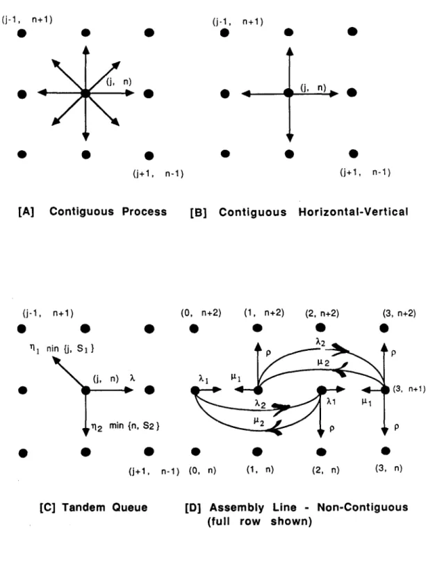
Examples To motivate the analysis that follows and indicate the prevalence of such row-continuous processes, some examples are appropriate. Transition diagrams for these examples are given in Figure 1.1.

A. Contiguous Processes

Any chain B(t) = [J(t), N(t)] on B =

{(j,n)\

0 ~ J' ~ J, 0 ~

n

~ N} for which

v(j,n),(k,m)

=

0 if

\i -

ki

>

1 or \m -

n\

>

1 will be called contiguous. The row-continuous chains are more general in that the marginal column process J(t) need not be skip-free.

For any contiguous process the transition rate matrices of (1.2) are tri-diagonal. All such processes that are irreducible are amenable to the methods we describe.

B. Contiguous Horizontal-Vertical Processes

A subset of the contiguous processes is of interest for which either J(t) or N(t) can change in a lattice continuous manner, but not both simultaneously. If, for example, J(t)

and N(t) were independent truncated birth-death processes, B(t) would be horizontal-vertical, since the probability of simultaneous change would be zero. In some cases, the independence between J(t) and N(t) may not be present, e.g. where J(t) is a truncated birth-death process and N(t) is a dependent birth-death-like process for which the upward and downward transition rates change when J(t) changes. One example of this type is a communication link carrying both voice and data[2]. We note that for such processes ~~

and ~;; are diagonal.

C. Tandem Queues with Blocking

A contiguous process of interest is the tandem two station queue where each station has finite waiting room, arrivals are Poisson with rate

.x,

and service times are exponential with service rates 111> 112. For this process v+ is diagonal, _=n ~-_-nis upper diagonal, and ~o _-n

is lower diagonal. (A matrix g

=

[aij] is upper diagonal if aij

i=

0 implies J'

=

i

+

1.)

The methodology treated here allows each station to consist of a finite number of servers. Various types of blocking and feedback could as easily be analyzed. Extensive numerical analysis and further discussion of this tandem queue model can be found in Section 7. D. Assembly Line

One interesting non-contiguous process is an assembly line with two machines in tan-dem and a buffer with finite storage in between. The marginal process J(t) describes fluctuating working and non-working states of the two machines, Ml and M2 which are governed by failure rates 11-1, 11-2 and repair rates

>'1, >'2

respectively. The two machines process work at the same rate of speed, i.e. have a common hazard rate p for completing their operation. When the second machine is down, items accumulate in the buffer. When the first machine is down, the flow of incoming items is cut off and the second machine goes idle after the buffer is emptied. The first machine stops when the buffer is full. N(t)

is the number of half-finished items in the buffer. For this model, both ~~ and ~;; are diagonal with two non-zero elements. The transition rate matrix ~~ has a zero diagonal.

(5)

(j-1. n+1)

•

Row-Continuous Finite Markov Chains

•

0+1. n-1) (j-1. n+1)

•

295

•

0.

n)

•

(j+1. n-1)

[A]

Contiguous Process

[8] Contiguous Horizontal-Vertical

(j -1 • n+ 1)

(0.

n+2) (1 • n+2) (2. n+2) (3. n+2)

•

• _•

111 nin

U.

SI} _p 0. n) A. 1..1

•

(3. n+1) 112 min in. S2} p

•

(j+ 1. n-1 )

(0.

n) (1. n) (2. n) (3. n)

[C] Tandem Queue

[0]

Assembly Line - Non-Contiguous

(full row shown)

(6)

296 J. KeUson, U. Sumita and M. Zachmann

§2. Passage Time Densities

The description of the ergodic and dynamic behavior we will develop is based upon the passage time densities for the bivariate process. To exploit the skip-free feature of row-continuous processes, the passage times between states of adjacent rows are treated as building blocks. The focus on a row of states as an entity then gives rise to a matrix probability density function describing the joint distribution between the time of arrival at the adjacent row and the state reached, as a function of state of origin. From the passage time p.d.f.'s for adjacent rows one can then describe regeneration times for the states of a row and hence the ergodic probabilities. This will be clearer from the details of the development.

To discuss the passage time densities it will be useful to work with the lossy process

jn(t)

for row

n

on the set

{(j, n)}

for which other states of 8 (i.e., other rows) are absorbing. Let

P(j,n),(k,n)(t)

=

P[J(t)

=

kj

N(t')

=

n,

0 ::;

t' ::; t

I

J(O)

=

i,

N(O)

=

n]

and as for (1.5) let ~nn

(t)

=

[P(j,n),(k,n) (t)].

Since ft~nn

(t)

= -~nn

(t)gDn

+

~n (t)g~, we may rewrite P

(t)

in the from of

==nn

P

(t)

= exp{Q

t},

=nn

=n

(2.1)

where

Q

n is the Q matrix for the lossy process, Le., Q- -

-1/

+

I/0

=n -

=Dn

=n

(2.2)

Note that ~nn(t) is strictly substochastic. Form (2.1) one then has for

itnn(s)

=

L[~nn(t)],

(2.3) The chain

B(t)

is uniformizable [10] in the sense that there exists a positive constant

1/

such that 00

>

1/

>

II?-ax

L

I/(j,m),(k,n)

since

J

and

N

are finite. If we let

(J,m) (k,n)

we have from (2.3) 1 1 1

a+

=

-1/+ . a-

=

-1/- . aO

=

1-

-[1/

- I/0]

=n

I/=n' =n

I/=n' ==n

==

1/ =Dn

=n

(2.4)

(2.5)

To proceed further, we require the passage time densities and some associated notation. Let s~:jk(T) be the joint probability density that, given one starts at

(j,n),

a) the row

(n+

1) is visited for the first time at time

T

and b) the row is visited at (k,

n

+

1). One then has

L

10

00

s~:jk(r)dT

=

1. Similarly, let

s;:jk(r)

be defined with respect to visiting the

k

row

(n-1)

for

n

~ 1. The irreducibility of

B(t)

implies that ~~(T)

=

[S~:jk(T)] and ~;(T) =

[s;'J'k(T)]

are matrix p.d.f's, see Definition 1.1. Correspondingly,

s+

= [00

~+(T)dT

and

. ==n

10-n

~;

=

10

00

(7)

L[~~(r)j and g~(8) = L[~~(r)j, and moment matrices ~:

(Xl

r§.-(r)dr,

one has

10

-n d p.-

=

--d

Q.n-(8)ls=0 .

=n 8 -297 (2.6a) (2.6b) The skip-free feature of the row-continuous processes provides a recursion between the upward passage time p.d.f.'s ~(r), and a recursion between the downward passage time p.d.f.'s ~~(r). There are direct matrix counterparts to those present for birth-death processes with J = {a}. The recursion is based on an argument similar to that employed in [7,8,lOj. For

N(t)

to go from n to n

+

1, it must either do so directly after motion on row n, or there must be a first downward transition to row n -1, a first subsequent return

to row

n,

and then a first subsequent arrival at row

n+

1. A probabilistic argument based on this then gives our basic recursive equation

~~(t)

=

~nn (t)g~

+

~n (t)g~

*

~~-l (t)

*

~~(t), n ~

1 (2.7) where the asterisk denotes convolution in time. That is,

~(t)

*

g(t)

=

f

~(t

- r)g(r)dr.

Consequently, from (2.7) and (2.4), we have

g~(8) = /I~nn(8)~~

+

/I~nn(s)~~g~-l (8)g~(8), n ~ 1. (2.8)

If we solve (2.8) for g~(8) and use (2.5), we obtain

/I 0 /I

[1 - (--){a

+

a-O'+ (s)}jO'+(8) = (--)a+.

= 8

+

/I =n =n==n-l =n 8

+

/I =n (2.9)

When n =

a

one has from ~t(t) = ~o(t)~ and (2.5) that

/I 0 /I

[I - (--)a jO'+(s) = (--)a+.

= 8+/1

=0=0

8+/1 =0 (2.10)

Equations (2.9) and (2.10) can be used to generate g~(8) recursively. Similar equations generate g~(8) recursively from

giV(8),

see(4.2). By letting

8

=

a

we obtain:

(2.11)

and

(2.12) Similar relations for !~ are given in (4.4). Differentiation of (2.9) and (2.10) with respect to 8 at 8 =

a

leads to the following relations for the mean first passage times:

(8)

298 J. Keilson, U. Sumita and M. Zachmann and

(2.14) We note that both ~~ and (~~ + ~;

+

~~) are stochastic. Since ~~ is not a zero matrix because of irreducibility, the matrix (~~

+

~; ~~-l) is strictly substochastic, its spectral radius is less than one, and

Ll: -

~~

-

~;~~-l] is invertible. One may therefore obtain ~~ from (2.11) and ~~ from (2.13). We also see that

Q,

S

~(s)

S

~~ and

I//(s

+

1/)

S

1 for

S

>

0 real. Hence

[1; -

(8~V){~~

+

~;g~_l(s)}] is invertible for

S

2:

0 real. Therefore (2.9) may be used to obtain gn +(8).

Of frequent interest in applications is the matrix passage time p.d.f. ~n (r) de-scribing the distribution of the time at which row n is first reached given a start at row O. Specifically ~n(r) is

[SOn:ij(r)]

where

SOn:ij(r)

is the joint probability density that the set {(j, n) : j E J} is visited for the first time at

(j,

n) and the time of first arrival is r, given a start at (0, i). A simple probabilistic argument shows that ~n(r) = ~(r)

*

~i(r)

* ... *

~~-1

(r).

Correspondingly, ~n(s) =

gt(s)gi(s) ..

·g~_l(s), This will be discussed further in Section 6.

§3. Ergodic Probabilities

We can now use the passage time densities of Section 2 to find the ergodic probabilities. The basic probabilistic argument for finding the transition probabilities from the passage times goes as follows. If one is in row n at time 0, to be in row n at time t, either

a) one never left row n;

b) one went to row n

+

1 before row n - 1, returned to row n for the first time subsequently, and was in row n at time

t,

possibly after further wanderings; or

c) one went to row n - 1 before row n

+

1, etc. as in b).

Consequently, one has, for the cases 0

<

n

<

N, n = 0, and n = N respectively,

and

e:NN(t)

=

gNN(t)

+

I/gNN(t)~N

*

~iv-l (t)

*

e:NN(t).

(3.3) From (3.1) it follows that

(9)

Row-Contimtous Finite Markoll Chains 299

One then finds, from (2.5), that

() ( 1 )[1 ( v ){ 0

+ -

()

- +

()}]-l

11" 8

= - -

- - -

a +a ~ 8

+g

a 8 .

=nn 8

+

V = 8

+

v, =n =n-n+l -n=n-l (3.5)

To show that the matrix expressed within brackets is in fact invertible, we let

E!n

(8)

=

(8:

v){~~

+

~~+l

(8)

+

~~g~-l

(8)) n

=

1, ... , N -1. (3.6) Note that (~~

+

~~

+

~;) is stochastic, and further

(3.7)

Therefore each row of

en

(8) is a convex combination of rows of matrix p.d.f.'s. Hence

[I -

(3

(8)]

is invertible for

8 >

0 real. With this identification, Equation(3.5) becomes

- =n

. 11" () 8 = - -( 1

)1'

1-(3

( )]

8 - . 1

=nn 8

+

1/= =n (3.8)

In fact, with the definition

(3.9a) and

(3

(8)

= (_V_)[aO

'+

a- a- (8)]

=N 8

+

1/ =N =N=N-l (3.9b)

we immediately obtain (3.8) for all nE N.

To find!!.~ we must evaluate lim 8Z[ (8) = 1e~. In [9] it is shown that

8-+0+ -nn

(3.10)

where !!.fn is the stationary left eigenvector for

en

(0) and ~n is the mean of gn(t), that is

and

I.L =

(>0 t/l (t)dt.

=bn

10

-n

(3.11)

(3.12) We can easily find (3 (0) by setting 8

=

0 in (3.6), (3.9a) and (3.9b), while I.L is accessible

~ =bn

by differentiation via

and

1

~o

=

v~(O)

+

~~~

(3.14)

As we will see in Section 5, row balance

(10)

300 J. KeiJson, U. Sumita and M. Zachmann

is always present. This enables one to evaluate T

mbn = l.I~nJ-L _=Iln

1

recursively without computing J-L ,and thus J-L+ and J-L-, in the following manner.

=bn =n =n

(3.10) one has !:.~

=

rn~n

ifn

so that

T - 1 T

-e a 1 = - - - e a 1

-n+1=n+1-

Q),n+1=n+1-mb,n+1

Hence, from (3.16), one sees that

T - 1 (3.16) From (3.17) ~ n+lgn+l-mb,n+l = mb,n 'T +1 0 ~ n ~ N - L (3.18) !:.b,ngn

One may start with an arbitrary positive mbO and then normalize at the end. More specifically, and mbO

>

0 , arbitrary [ ' " 1 T ]-1 K= ~ --~nl . nEJJ mbn

§4. Summary of Computational Procedures

(3.19)

(3.20)

A tabulation of the key results obtained in the previous sections is given to provide an overview of the formalism, and ease of access to the formulae needed for implementation.

(4.1)

- ()

[

(1.1)

0 ]-1( 1.1 ) _

a S = 1- - - a - - g,

=N = S+I.I =N s+I.I-N

(4.2)

o'-(s) =

[1 -

(_I.I_){ao

+

a+O'-

(s)}]-l(-I.I-)a-=n = S

+

1.1 =n =n=n+1 S

+

1.1 =n

(4.3)

(4.4)

(11)

Row-Continuous Finite Markov Cluzins

- 1

[f

0 ]1 -gN=~=-g"N gN

g: =

~[L

-

{g~

+

g~~+1)}r1[L

+

vg~g:+l}]g~

f3

(s) = (_v_)[aO

₊

_a+o- _(s)

₊

_{a-a+ (s)]}

=n S

+

V

=n

=n='n+1

=n=n-1

1 _ 7r

_{nn (s)}

=

( - ) [ l -

f3

(s)] 1

s+V·-

=n mbn = mb.

n-1 (

T

+

) ,

~.n-1gn-11 T K T ~n = --~n mbn

§5. Row Balance and Row Generation

mbO

>

0 arbitrary 301

(4.6)

(4.7)

(4.8)

(4.9)

(4.10)

(4.11)

The computational procedure outlined in Section 3 and 4 is a rank-reducing procedure. The procedure can further be improved by using set balance on the state space, when mean passage times are not needed. A still greater improvement can be realized when the ~

(or g~) are invertible for all n. We have seen in Section 1 that the required invertibility is often present.

To exhibit row balance, some preliminary tools are needed.

Lemma 5.1

(5.1)

and

T - T[f 0]

~l

f!1

=

~ =: -

f!o .

(5.2)

Proof: The forward equations are:

d

dt1!.~(t)

=

-V1!.~(t) +V1!.~(t)~ + V1!.~_1(t)g~_1 +V1!.~+l(t)f!~+l'

1:5 n:5 N -1 (5.3)

and

(12)

302 _{J. Keilson". U Sumita and M. Zachmann}

Since l!.~(t) -+ ~,!:, and

-itlli(t)

-+ QT as t -+ 00, the result is immediate.

Theorem 5.2 If _=na- is invertible for all 1

<

_- n

<

_- N then

~'!:+l = {~'!:L! - ~~]- ~~-1~~+l}(~~+l)-1, 1

S

n

S

N - 1 (5.5) and

T T[I 0]( -)-1

~1 = ~ = - ~ ~1 • (5.6)

Proof: The theorem follows directly from (5.1) and (5.2).

We see that when the ergodic distribution is desired, and this invertibility present, the ~'!: are available recursively via (5.5). In such a case, one needs to calculate only one eigenvector (~ro) in order to obtain the other ~'!: recursively.

A similar result holds when ~~ for 0 S n SNare invertible. The recursion then begins with ~t.

and

Theorem 5.3 If ~n is invertible for all n >0 theri

~'!:-1

=

{~'!:L!

-

~J

-

~'!:+1+l}(_1)-1

, T _ T

[I

0

l(

+ )-1 ~N-l - ~N = - ~N ~N-1 .

n= 1, ... ,N-1

(5.7)

(5.8)

Proof: Equation (5.7) follows by rearranging (5.1). The forWard equation (5.4) has its counterpart on the top row

:tl!.~(t)

=

-Vl!.~(t)

+

1Il!.~(t)~~

+

1Il!.~_1 (t)~Jt._1·

By letting

t

-+ 00, (5.8) follows from (5.9).

(5.9)

Even when neither set is invertible, set balance can be used to normalize the

ifn'

as described at the end of Section 3. We are now ready to prove our basic result regarding the set balance.

Theorem 5.4 (Row Balance)

T

1-

T +1

-'n+l~n+l -

-'n

~n for 0

S

n

S N

-1 .

(5.10)

Proof: We recall that ~~1 = 1-(g~

+

~)l and ~1 = 1-~l. Combining this with Lemma 5.1 we obtain

T +1 T - 1 - T + 1 T -₁

~n~-- ~n~n+l-- ~n-l~n-l-- ~ngn- (5.11)

and

T +1 T -₁

~ ~o - = ~1 ~1 -' (5.12)

(13)

Row-Continuous Finite Markov Cha,ins 303

§6. The Matrix Polynomial Representation of ~n(s)

Important information on the dynamical behavior of a Markov chain is contained in the spectral structure of its first passage time densities. Knowledge of this structure, and that of the related relaxation time, is essential when one wishes to use the ergodic distribution [10]. In this section, we discuss a representation of

gmn(s)

in terms of matrix polynomials, where the set of poles of

gmn(s)

corresponds to spectral lines.

Our approach closely parallels the work done on one-dimensional birth-death process in [5,6] and [7,8,10]. This representation will be used to discuss the structure of ~On(T) and simple related results. We also indicate how this representation may be used, in principle, to obtain the relaxation times.

Theorem 6.1 If ~~ is non-singular for all n, let

+ 1 S+1I

°

2n+1(s)

= (~n)- [{(-II-)b--~}Qn(s) -~;;-2n_1(s)] (6.1) with

Q (s)

=

I

j Q (s)

=

(g+)_1[(S

+

lI)l -

aD].

==0 - =1 -11 11 - =0

(6.2)

Then the matrix polynomial Q (s) is invertible for s

?

0, and =n

u;t-(s)

=

Q (s)Q-1 (s).

=n =+1 (6.3)

Proof: We prove the theorem by induction. Clearly Q

1(s) = C~/I)(~)-l[L

(~)~] where ~ is strictly substochastic. Hence

Q1(s)

is invertible for all

s

?

O. Thus (6.3) holds true for

n

= O. Now assume that

q

(s)

is non-singular for 0 ~

n

~ M and

==n

u;t-(s)

=

Q (s)Q

(s)-1

for 0 ~ n ~ M -1. Then

=n =+1

Since

gt_1(s)

is the transform of a matrix p.d.f., we see that

QM+1(s)

is invertible for

s

?

o.

Postmultiplying (6.4) by

Q;}(s)

and inverting one sees from (2.8), that

gt(s)

=

Qu(s)Q

(s)-1,

completing the proof.

=<... -d!:M+1

We note that the recursion relation (6.1) implies that Q (s) __ is a polynomial in s of =n '3

degree n. The decomposition (6.3) will be seen to be useful in a variety of ways.

The (Q (s)) if arrays allow one to evaluate first passage times upwards and downwards =n

over a number of rows rather easily. The following theorems illustrate this point.

Theorem 6.2 In the context of Theorem 6.1, one has :

(14)

304 J. Keilson, U. Sumita and M. Zachmann

b)

Q~+l

(0)

= (~~)-1{(~)2n

(0)

+

(l-

~~)Q~(O) - ~~Q~-l

(O)}

with

~(O)

=

~

and

Q:

(0) =

~~-lj

(6.6)

c)

~n = Q:l(O)Q~ (O)Q:l(O).

Proof: We observe from Theorem 6.1 that

n-l n-l

gon(s)

=

11

~(s)

= 2o(s)(

IT

Q:1(s)Qm(s))Q:1(s)

=

Q:l(s),

m=O m=O

proving (a). For (b), we see from (6.2) that for n 2: 2,

Part (b) then follows for n 2: 2 by setting s = O. The cases for n = 0,1 are trivial. We note from (a) that Q

n

(s )~n (s)

=

l.

It then follows that

(6.8)

Therefore, one has

(6.9)

proving (c).

Theorem 6.2 provides a computationally easy way to calculate the mean upward pas-sage times when ~~ are invertible. A dual argument eases the computation of downward passage times when ~ are invertible. The explicit formulation for arbitrary upward passage times is given next.

a) b) Theorem 6.3 ~n(s)

=

2m(s)Q;l(s)

for 0 ~ m ~ n ~ N J1,

=

Q (O)Q-l(O)Q' (0)Q- 1(0) - Q' (0)Q- 1(0)

for 0 ~ m ~ n ~ N

=mn

=m

=n

=n =m =n (6.10)

(6.11)

Proof: Since ~m(s)~n(s) = ~n(s), part (a) follows from (6.5). From (a), we see that ~n(s)Qn(s) =

Qm(s).

By differentiating this at

s

=

0, one finds that

(6.12) From (a) and the identity

_=mn

J1, = -Q'

_-mn

(0), statement (b) now follows.

We note that

Q+(s)

=

Q (s)Q-1 (s)

implies that

-n

=n

==n+1

~+ =

Q (0)Q-1 (0).

-n =n

=+1

(6.13)

Thus, calculation of Q (0), and Q' (0) is sufficient to give ~ and J1, directly.

=

=n

-mn

=mn

The matrices Q (0) and Q' (0) can be calculated recursively using (6.1) and (6.6)

=n

(15)

Row-Continuous Finite Markov Chains 305

and mean stationary sojourn time, two useful measures of the dynamical behavior of the queue [10]. Both are defined with respect to a partition of the state space into two disjoint connected sets, called the good set and the bad set.

The ergodic exit time is the time required to leave the good set given that the system has reached its stationary state and is in the good set. Let a partition of the state space be defined by,

Gm

=

{U,

n) : n

<

rn} , Bm

=

{(i,

n) : n

2:

rn}.

Since entry into Bm is at row rn, the mean ergodic exit time from Gm, denoted by ILEm, is given by

(6.14)

Using Theorem 6.3, this then leads to

(6.15)

The stationary sojourn time from Gm is the time required to first leave the good set given that the system was stationary and a transition into the good set from the bad set just occurred. The mean stationary sojourn time ILvm is given by

(6.16)

This can be rewritten in a simpler form using a well known result [10] as ILVm

=

~oo(~

BmGm

where Poo ( Gm) is the total ergodic probability on the set Gm, and iBmG_{m is the ergodic}

probability flow from Bm to Gm. It then follows that

(6.17)

§7. A Tandem Queue Example

A tandem queue is a queueing system with distinct service facilities connected in series, i.e. the customer output stream of the first facility is the input stream of the second [13]. To illustrate the algorithmic procedure we have developed, one such tandem queue will be analyzed. The example selected has been chosen primarily for didactic reasons. A more complex and realistic example could have been analyzed with little increase in computational time.

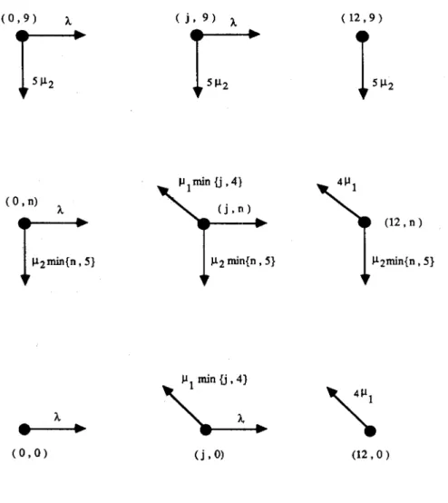
The tandem queue evaluated is a two server series queue with blocking and finite buffers, see Section 1, Example C. The first service facility has 8 buffer slots and 4 servers. The second facility has 4 buffer slots and 5 severs. A flow diagram is given in Figure 7.1.

(16)

The corresponding rate matrices are given in Figure 7.2. When the first queue is full, customers balk and go elsewhere. When the second queue is full, the first queue stops serving until a space at the second facility becomes available. The model can easily be modified to allow different types of blocking, and features such as feedforward, feedback, etc.

In Figure 7.1 the occupancy level at the first facility is given by the coordinate

i

which corresponds to the number of people in service or waiting there. The occupancy level at the second facility is given by the coordinate n. The blocking may be seen in the absence of the transition rates associated with 1-'1 on the top row.

Figure 7.2 displays the three matrices ~~, ~,and~;; when n = 3. The matrix ~~ is upper diagonal for all n. The only transitions which have no impact on the second queue

are the arrivals (at rate

>.)

to the first queue, which increase that occupation level by one. The matrix~;; is diagonal, with diagonal elements 1-'2

=

min{n,

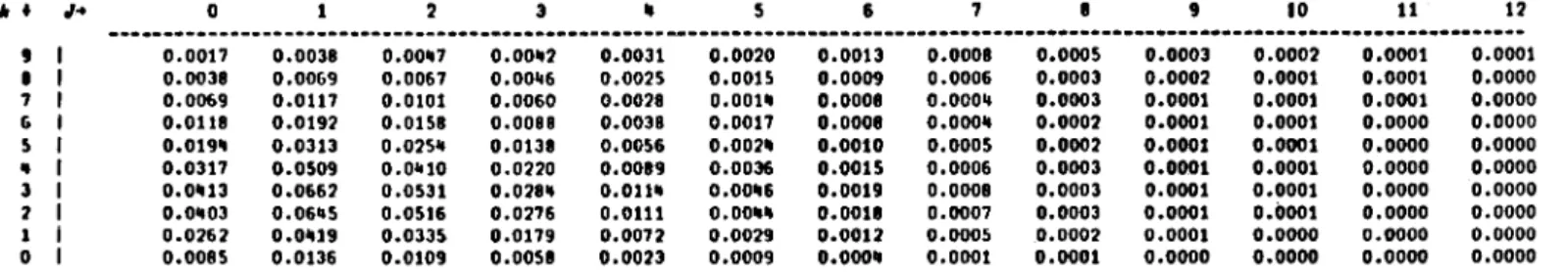
k2} where k2 is the

number of servers in the second service facility. Finally, ~~ is lower diagonal. Increases in queue length at the second service facility are caused by departures from the first facility. The results are shown in Figures 7.3 (a), (b), (c), 7.4 and 7.5 for a traffic intensity of 0.4 at the first facility and 0.6 at the second. Figures 7.3 (a), (b), (c) describe the ergodic probabilities as a function of

(i,

n). An examination of these figures immediately reveals two features. First, the ergodic probabilities are significant for modest values of

i

and n,

arising from the moderate traffic intensities. The small ridge visible along the upper edge of Figure 7.3 (a) indicates some blocking.

The ergodic probabilities may be useless when system parameters change before er-godicity is reached. The information contained in the first passage times may then be helpful. The ergodic distribution, for example, might cause concern over large probabili-ties of saturation, blocking, long waiting times and so on. From the last table in Figure 7.5 describing the mean first passage times from idleness, we see that the mean time to saturation is on the order of 4 days provided that our time scale is in hours. If this queue modeled a system that starts anew each day, one would be less inclined to worry.

The tables in Figure 7.4 give, for differing levels, the mean sojourn time, i.e., the mean time spent above a certain level after the level is reached. This gives a feeling, for example, for the persistence time in a congested state. The first two tables in Figure 7.5 present mean first passage times one step upward (downward). The

(i,

n) entry in the table is the mean time to go from

(i,

n)

to a state in the row

n

+

1

(n -

1). Again, the effect of blocking is noticeable in the drop off (for the upward table) of the passage time with increasing values of i.

(17)

(0,9) A

r.-(0, n) A

I"2mm{n~'J

A

•

(0,0)

( j , 9 ) A

r.-(j,n)

----'

...

112 min{n , 5}

C

(j , 0) ( 12,9 )

~

(12,0)

Fig. 7.1

Transition Rate Structure For The Tandem Queue

307

Transition rates are shown for representative edge, coner, and

interior states.

(18)

308 J. Kei/son. U. Sumita and M. Zachmann 0 A 0 0 0 0 A 0 13 x 13 ,,0 = =n 0 A 0 0 0 A 0 0 0 31-'2 0 0 0 31-'2 0 0 31-'2 13 X 13

_!fi=

₀ 0 0 0 31-'2 0 0 1-'1 0 0 _2"'1 0 13 X 13 _~,,+

=

₀ _31-'1 0 41-'1 0 0 41-'1 0

(19)

"

.

r/oO 9

•

7 6 5

..

3 2 1 0

TANDEM QUEUE EXAMPLE

SIZES: BUFFER (1) = 08 BUFFER (2) = 04 SERVES (1) = 04 SERVES (2) = 05

ARRIVAL RATE = 4.000 SERVICE RATE (1) = 2.500 SERVICE RATE (2) = 1.300 ERGODIC PROBABILlTlES 0 2 3 11 5 6 7

•

9 10 11 12

---.---_.---._---.---

0.0017 0.0038 0.00"7 0.00,.2 0.0031 0.0020 0.0013 0.0008 0.0005 0.0003 0.0002 0.0001 0.0001 0.0038 0.0069 0.0067 0.00"6 0.0025 0.0015 0.0009 0.0006 0.0003 0.0002 0.0001 0.0001 0.0000 0.0069 0.0117 0.0101 0.0060 0.0078 0.00111 0.0008 0.00011 0.0003 0.0001 0.0001 0.0001 0.0000 0.0118 0.0192 0.0158 0.0088 0.0038 0.0017 0.0008 0.000" 0.0002 0.0001 0.0001 0.0000 0.0000 0.01911 0.0313 0.025" 0.0138 0.0056 0.002" O.OOtO 0.0005 0.0002 0.0001 0.0001 0.0000 0.0000 0.0317 0.0509 0.0"10 0.0220 0.0089 0.0036 0.0015 0.0006 0.0003 0.0001 0.0001 0.0000 0.0000 0.0"13 0.0662 0.0531 0.02811 0.011" 0.00"6 0.0019 0.0008 0.0003 0.0001 0.0001 0.0000 0.0000 0.0"03 0.06115 0.0516 0.0276 0.0111 0.00 .... 0.0018 0.0007 0.0003 0.0001 0.0001 0.0000 0.0000 0.0262 0.0"19 0.0335 0.0179 0.0072 0.0029 0.0012 0.0005 0.0002 0.0001 0.0000 0.0000 0.0000 0.0085 0.0136 0.0109 0.0058 0.0023 0.0009 0.000" 0.0001 0.0001 0.0000 0.0000 0.0000 0.0000

Fig. 7.3(a) The Ergodic Probabilities

For The Tandem Queue Model

~ 0 ~ ~ ::s ~. ~

..

~

~.

~

...

~

s·

..

'""

C '0

(20)

(9,0)

(0, 12 )

n

(O,O)

Fig.7.3(b) The ergodic probabilities

for the tandem

queue model

(9,0)

n

0.001

(0,0)

( 0 , 12)

(21)

MEAN SOJOURN TIMES ON THE SET { (J,N) :

N

~

X }

x •

~ 3

-

5 6 7

•

9

---_._---5.6001116 1.568603 0.1680115 0.496111 0.39221_ 0.319189 0.347591 0.2119_9 0.153846

MEAN SOJOURN TIMES ON THE SET { (J,N) : J ~

X }

x •

2 3

"

5 6 7 8 9 10 11 12

0.039110 0.0111885 0.009001 0.001106 0.001581 0.00817" 0.00'83~ 0.0091130 0.009751 0.0091183 0.008210 0.0053111

Fig. 7.4 The Mean Sojourn Time

For The Tandem Queue Model

::tI c ~ ~ ;:s ~.

s

§l

~. ~

~

'"

~

s·

'"

"'"

... ...

(22)

""

"-MEAN RRST PASSAGE TIMES ONE STEP UPWARDS (t N) w

11 • J+ 0 2 3 11 5 6 7

•

9 '10 11 12

._.---._---•

18.1602 12.3717 7.716" ".6200 2.7606 1.96'" 1."'50 1.162' 0.9357 0.7732 0.65911 0.5'70 0.553" 7 11.3:l9" 7."297 ".6352 2.7777 1.6617 1.181" 0.8929 0.702" 0.5721 0.1182" 0."219 0.38"7 0.3678

"

6.7328 11.3919 ).7236 1.6223 0.9665 0.6860 0.5235 0."225 0.3583 0.317" 0.2919 0.2771 0.2707 5 3.91176 2.5233 1. 5257 0.8898 0.5278 0.3828 0.3078 0.2670 _0.2""" 0.2319 0.2251 0.2211; 0.2202

..

2.2708 1.35"2 0.7750 0 ... 33 0.2735 0.2U6 0.1958 0.1859 0.1816 0.1797 0.1789 0.1786 0.1785 3 1."271 0.7981 0 ... 51 0.2636 0.1786 0.1590 0.1531 0.1513 0.1507 0.1505 0.1505 0.1505 0.1505 2 0.9615 0.5103 0.2888 0.18"6 0.131" 0.1308 0.1296 0.129" 0.129" 0.12911 0.12911 0.129" 0.129" 1 0.6831 0.3502 0.2092 0.1"51 0.1150 0.1131 0.1130 0.1130 0.1130 0.1130 0.1130 0.1130 0.1130 0 0.5055 0.2555 0.1652 0.1217 0.1000 0.1000 0.1000 0.1000 0.1000 0.1000 0.1000 0.1000 0.1000 ~ ~

MEAN RRST PASSAGE TIMES ONE STEP DOWNWARDS (~N) ;:., _~

;:s 11 • J+ 0 2 3 11 5 6 1

•

9 10 11 12 _!=:: ---~---_._---_

..

---

~ 9 I 0.1538 0.1538 0.153' 0.153' 0.153' 0.1538 0.1538 0.1538 0.1538 0.153' 0.1538 0.1538 0.1538 _;: 8 I 0.18"8 0.2351 0.2839 0.3295 0.3612 0.3816 0.3811 0.3892 0.3900 0.3903 0.3905 0.3905 0.3905

i"

1 I 0.1915 0.2685 0.3516 0."581 0.5582 0.6226 0.6659 0.6950 0.11115 0.1275 0.1362 0.71117 0.7 ...

..

6 I 0.2033 0.2836 0.3920 0.5267 0.67"8 0.189" 0.8820 0.9579 1.0202 1.0711 1.1121 1.1"39 1.16"8

5.

5 I 0.2051 0.2900 0."068 0.5573 0.7307 0."66 1.00"3 1.1180 1.2198 1.3101 1.3907 1."583 1.5065

..

I 0.2728 0.3773 0.5185 0.6971 0.9021 1.085" 1.2535 1."103 1.55711 1.6951 1.822_ 1.93". 2.0115 ~ J I 0."333 0.6057 0.8166 1.0622 1.3279 1.5609 1.7811 1.9925 2.1963 2.392" 2.5782 2.7"57 2.8699 _~ 2 I 0.9_27 1.3055 1.6983 2.1009 2."89. 2 •• 0 .. 6 3.0961 3.3773 3.6516 3.9116 11.17112 11."057 ".5761 _g. 1 I 11.0319 5.0923 6.0317 6.8311 7 .... 29 7.9339 '.3233 '.6893 9.0"36 1.3862 1.7177 10.01'13 10.2292 ~

.,.

MEAN RRST PASSAGE TIME FROM IDLE TO GIVEN N

2 3 11 5 6 1 8 9

---_

... ---_.-.-

..

_.---0.5055 0.9382 1."672 2.2167 3.'1175 5.5906 9.3"70 15.6818 26.2116

Fig.7.S The Mean First Passage Times

(23)

Row-Continuoulf Finite Markov Chains 313

Acknowledgment

The authors wish to thank the referees for helpful comments, S. Grav~s for useful discussions and Y. Ishikawa for his extensive editorial assistance.,

References

[lJ Cinlar, E., "Markov Renewal Theory: A Survey," Management Science, Vo1.21, pp.727-752,1975.

[2J Friedman, D., "Queueing Analysis of A Dynamically Shared Voice-Data Link", Ph.D. Thesis, Department of Electrical Engineering and Computer Science, M.I. T, 1981.

[3J Gaver, D. P., Jacobs P. A. and Latouche, 'G., "Finite Birth-and-Death Models in Randomly Changing Environments," Advances in Applied Probability, V01.16, pp.715-731,1984.

[4J Hajek, B., "Birth-and-Death Processes on Integers with Phases and General Bound-aries," Journal of Applied Probability, VoLl9, ppA48-499, 1982.

[5] Karlin, S. and McGregor, J. 1., "The Differential Equations of Birth-and-Death Processes and the Stieltjes Moment Problem" , Transactions of American Math-ematical Society, Vo1.85, ppA89-546, Hl57.

[6] Karlin, S. and McGregor, J. L., "The Classification of Birth and Death Processes", Transactions of American Mathematical Society, Vo1.86, 1957.

[7] Keilson, J., "A Review of Transient Behavior in Regular Diffusion and Birth-Death Processes", Journal of Applied Probability, VoLl, pp.247-266, 1964.

[8] Keilson, J., "A Review of Transient Behavior in Regular Diffusion and Birth-Death Processes - Part Il", Journal of Applied Probability, Vo1.2, ppA05-428, 1965. [9] Keilson, J., "On the Matrix Renewal Function for Markov Renewal Processes", The

Annals of Mathematical Statistics, Vo1.40, pp.1901-1907, 1969.

[10] Keilson, J., Markov Chain Models - Rarity and Exponentiality, Springer-Verlag, New York, 1979.

[11] Keilson, J. and Wishart, D. M. G., "A Central Limit Theorem for Processes De-fined on a Finite Markov Chain," Proceeding of the Cambridge Philosophical Society, Vo1.60, pp.547-567, 1964.

[12] Keilson, J. and Wishart, D. M. G., "Boundary Problems for Additive Processes De-fined on a Finite Markov Chain," Proceeding of the Cambridge Philos<,?phical Society, Vo1.61, pp.173-190, 1965.

[13] Kleinrock, L., Queueing Systems, Vol. 2: Computer Applications, John Wiley & Sons, New York, 1976.

[14] Neuts, M. F., "Markov Chains with Applications in Queueing Theory Which Have a Matrix-geometric Invariant Vector", Advances in Applied Probability, Vol.l0, pp.185-212, 1978.

(24)

314 J. KeUson. U. Sumita and M. Zachmann

[15] Neuts, M. F., Matrix Geometric Solutions in Stochastic Models - An Al-gorithmic Approach, The Johns Hopkins University Press, 1981.

[16] Pyke, R., "Markov Renewal Processes: Definition and Preliminary Properties," Annals of Mathematical Statistics, Vo1.35, pp.1746-1764, 1964.

[17] Schweitzer, P., "Aggregation Methods for Large Markov Chains," Invited Paper in the Proceedings of Mathematical Computer Performance and Reliability, P. J. Courtois and A. Hordijk (editors), pp.275-286, 1984.

[18] Takahashi,Y., "A Lumping Method for Numerical Calculations of Stationary Dis-tibutions of Markov Chains," Research Report B-18, Department of Information Sciences, Tokyo Institute of Techinology, Tokyo, Japan, 1975.

[19] Takahashi, Y. and Takami, Y., "A Numerical Method for the Steady-State Proba-bilities of a GI/G/C Queueing System in a General Class," Journal of Operations Research Society of Japan, Vo1.19, No.2, pp.147-157, 1976.

Ushio SUMITA: William E. Simon

Graduate School of Business Administration, University of Rochester,