A Computational Method for Dynamic Linear Programming

(1)

A COMPUTATINAL METHOD FOR DYNAMIC LINEAR PROGRAMMING

TAKESHI FUKAO

(Electro-technical Laboratory)

(Presented at the 4 th meeting November 16, 1958)

(Received October 5, 1959) 1. INTRODUCTION.

The dynamic linear problem, consisting in optimizing the cost (or measure of effectiveness) over some time period, consists of a sequential set of static problems which have nearly the same structures each other. Applying the standard linear programming technique to such a dynamic linear problem without noticing the above feature, the problem be-comes an in hi bitingly large linear programming problem, and this situa-tion is not desirable in view of the difficulties of computasitua-tions, and the necessity of higher accuracy of computational results, etc.

On the other hand, if we notice the above feature of dynamic pro-blem, and if we solve the problem following to some suitable sequential process, it is only necessary to solve many smaller, but nearly same structural linear programming problems, and the faults described above could be removed. A typical type of these sequential processes is the Bellman's dynamic programming, and the other typical one is the Danzig's dynamic linear programming method. (2) Although they are excellent general methods, there are some difficulties in application to the practical problems. That is, in Bellman's dynamic programming, the complexity of each static problem is an essential difficulty in computations, and it is necessary to invent some devices suitable to the problem in the Danzig's method.

In this paper we will describe a more natural computational method (one type of relaxation method) and its numerical examples, and we will touch on the extensions of the basic concepts of this method.

98

(2)

2. REDUCTION OF A DYNAMIC PROBLEM TO A MULTI· STAGE DECISION PROCESS (OR A GENERALIZED VARIATIONAL PROBLEM).

We define a multi-stage decision process (problem) as follows: 1) It includes decisions (variables) and states(variables), as shown in Fig.

1., and the relations

~: ~:i~::~:n

(1) F, F, F, F,

~!W4l+-=

So S. S, S, S,

L-l 1

~

1

o 1 2 4 hold,

2) the cost (measure of

opti-mization) of it is separable: Fig. 1.

F=Fj(So, Xl, SI)+P2(Sl, X2 , S2)+···, (2) and

3) the constraints are also separable:

~:i~::;:: ~:~~ ~

1

(3)

Where, Si describes a set of states at the i-th "time" (It is not necessary "time" is time. It is sufficient "time" is only an order number of the sequential state.), Xi, a set of decisions at the i-th stage, res-pectively. Dynamic programming is applicable to such multi-stage decision problems. Then it is necessary to transform a given problem to a pro-blem which satisfies the conditions (1), (2), and (3) by introduction of an adequate set of decisions and states, in order to be able to apply the dynamic programming concept.

Particularly, if we assume the linearities in conditions (1), (2), and (3), the problem becomes a linear programming problem, and its stru-cture is represented by the coefficients matrix form of the following equations (3'):

~:i~::~::~::~:i:~

)

(3')

Where, ).1, ).2··· .. · are slack va:riables.

(3)

100 Takeshi Fukao

owing to this coefficients matrix (technology matrix) form. These

discus-sions come largely from Danzig's paper. (2)

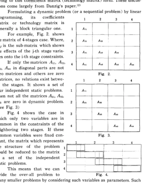
Formulating a dynamic problem (or a sequential problem) by linear

programming, its coefficients

matrix or technology matrix is generally a block triangular one.

For example, Fig. 2. shows

the matrix of 4-stages case. Where, 2

A i j is the sub-matrix which shows

the effects of the j-th stage varia- 3

bles onto the i-th stage constraints.

If only the matrices A1l , A22 , A33 , A44 in diagonal parts are not

zero matrices and others are zero matrices, no relations exist

betwe-en the stages. It shows a set of

four independent static problems. Then not all the matrices A2b A32 ,

A43 are zero in dynamic problem.

(See Fig. 3)

Fig. 4 shows the case in which only two variables are in common in the constraints of the

neighboring two stages. If these

common variables were fixed con-stant, the matrix which represents the structure of the problem would be reduced to the matrix

2 of a set of the independent

static problems. 3

This means that we can 4

divide the over-all problem to 4 2 3 4

I

,

I

An A21 I , All A" An A21 t

I

!

I

=

2 A22 I A" , A" Fig. 2. 2 A •• A" I Fig. 3. 3 4 A" A •• A .. 3 4 A" A .. A .. 2 3 4 ---1 _____ : i

I

I , I , , , , I [ , :! _:' Fig. 4.

many smaller problems by considering such variables as parameters. Such common variables are states (variables), and the remaining variables are decisions (variables). Number of these common variables or states variables becomes larger according to the higher dimensional system

(4)

and to the system including the time lag and acceleration effects. Then,

at last, the matrix may become I

(~

such as Fig. 5. In this case, it is necessary to consider two stages as one stage in the new problem in order to reduce the problem to a multistage deci-sion process.

Because the fewer states 2

3

4

5 6

are in a stage, the more easily Fig. 5.

the problem is dealt with, the central problem is how to obtain the more loosely-coupled matrix by the introduction of the suitable states and decisions.

3. ARBITRARINESS OF THE CHOICES OF STATES AND DECISIONS.

In Fig. 5 case, it was necessary to take two stages in the old pro-blem as one stage in the new propro-blem in order' to reduce the propro-blem to a multi-stage decision process.

Let us call the variables which the constraints of a stage and the constraints of the next stage have in common as the coupling variables. We designate the number of the coupling variables, the states, the deci-sions and the all variables of one stage, ne, n., nd, and n, respectively.

If

(K-l)n <: lie <: Kn, (4)

then it is necessary to take at least K stages in the old problem as one

stage in the new problem in order to reduce the problem to a

multi-stage decision process. If we take K

stages as one stage in the new phase,

under the condition K 2: 2, the rela- <I i'm:777:'*"""",.".,j----;---j---+--___j

" tion

nd ::;; n.( =nc) (5) exists. The equality is valid only when ne=n, that is, Fig. 6 case.

The fewer states are in a stage, the more effective a multi-stage

deci-~~~~~~""~--.--+---+---j

(5)

sion process is. That is, it is more effective when applied to the problem which has the week couplings between the stages. Moreover, when the couplings are stronger, the classifications of the states and the decisions are more and more artificial, and there are no physical differences between them at all.

In this situation, the application of the following relaxation method, based on a standpoint of taking K stages as one stage in the new problem only from the view point of the division of the variables (not necessarily from the view point of the division of the constraints), is more systematic and more effective sometimes in the stronger coupling problems.

Let us consider the Fig. 5 case, for example. We take the combi-nation of the I-st and the 2-nd stages in the old problem as the I-stage, the combination of the 3-rd and the 4-th as the II-stage, and the combi-nation of the 5-th and the 6-th as the Ill-stage, respectively, in the new division of the variables. See Fig. 5.

We assume that a multi-stage decision process MJ which has the variables of the odd stages (the 1-, the Ill-stages) as its decisions and the variables of the even stage (the II-stage) as its states, the another multi-stage decision process M2 , which has the variables of the even stage as its decisions and the variables of the odd stages as its states.

First, from a standpoint of MJ , the decisions of the I-stage are

determined independently of the Ill-stage decisions, preserving the vari-ables of the II-stage (states) constant, Next, from a standpoint of M2 , the decisions of the II-stage are determined, preserving the variables of the 1- and Ill-stages constant (using the newest informations). In the next place, from a standpoint of MJ again, the decisions of the Ill-stage are determined, preserving the variables of the II-stage constant. This processes are repeated again and again.

In this method, two kinds of multi-stage decision processes are used alternately, and corresponding to the kind of multi-stage decision process the variables of a stage are regarded as the decisions, and also as the states in the another one.

We should bear in mind that the division of the constraints do not necessarily correspond to the division of the variables. For example, in the above case, from a standpoint of M1, the decisions of the I-stage

(6)

are the variables of the I-st and the 2-nd stages of the old problem, but the constraints to these decisions are the constraints of the I-st, 2-nd, 3-rd and 4-th stages of the old problem.

This method is a relaxation method, and similar to the over-lapping method described in the following paragraph.

4. OVERLAPPING METHOD AND ITS AVAILABILITIES. Although this method is applicable both to the multi-stage decision processes (paragraph 2.) and its extensions (paragraph 3.), we shall ill-ustrate it with respect only to the former.

4-1. ONE FORM OF OVERLAPPING METHOD.

If a problem is reduced to a multi-stage decision process, the rela-tions between decisions and states are shown in Fig. 1, as already described.

Now, we take the successive approximations due to overlapping as follows:

The initial estimates of states are 50CO ), 51(0), 52 (0), 53(0), ...• ( i) The two-stages optimization problem of which boundary con-ditions are 50=50co

>,

52=52 (0), is

solved. The solution determines

51=51(1). See Fig. 7.

(ii) The two-stages opti-mization problem of which boun-dary conditions are 51 =51 (1), 53

(1) (1) (1) (1) (1) (1) S. 82 S. S. SN-2 SN-1

V',~~~

~~~-(0) (0) (0) (0) (0) (0) (0) (0) So 8. S2 S, S. SN-2 SN-1 SN

0----t-+--*3

--+;i----;N'."--'--;2"N"-'---' l.----1N Fig. 7.

=53

(°>,

is solved. The solution determines 52=52(1). See Fig. 7.

(iii) The two-stages optimization problem of which boundary conditions are 52=52(1), 5₄=5₄(°\ is solved. The solution determines 53= 53(1). See Fig. 7.

The similar step, that is, solving the two-stages optimization pro-blem using the newest 5 informations as its boundaries, and then moving one stage to the right, is repeated until getting 5N(1). Next,

again back to the initial two-stages optimization problem. These approxi-mation steps continue until all 5i have converged.

For the problems having free end states conditions, many modi-fications are possible. For example, modifying the end states 5N

(7)

gradually, taking a particular sub-problem of which boundary conditions

are SN-l =SN-l (n) without SN=SNln), etc.

The validity of this method is proved as follows. We consider a maximization problem, and we suppose the uniqueness of the solution for simplicity.

(1) Each step of "overlapping" (solving the two-stages linear pro-gramming) has monotone increasing property. From this property and the boundedness of the problem, it is clear to converge to some states. (2) We assume that So(l) is a series of states or a set of

argu-ment functions converged by overlapping method, and OSi,m(t) is a set

of variational functions which are zero before the i-th "time" and after the i+2-th "time".

Then, general argument functions are expressed by

N-2

S(t) =Soct)

+

~ OSi,i+2

i~O

Because the cost is linear with respect to decisions, and the rela-tions between decisions and states are linear,

N-2

cost (S(t)) =cost(So(t)) + ~ cost (OSi,i+2(t) )

i~O Now, the following conditions hold:

coSt(OSi,i+2(t));;;;;; 0 Ci=O, 1, "', N-2).

For if any cost (OSi,i+2) were positive, the overlapping method would

have not yet converged.

From (1) and (2), the optimality of So(t) has been proved.

There are many types of overlapping method which vary due to the number of stages of the sub-optimizing problems, the order of over-lapping (Non systematic overover-lapping is a general relaxation method for optimization problems.), etc. We can reduce the number of optimizing problems if we increase the number of stages of each sub-optimizing problem. The same proof is established for the extension of the multi-stage decision process(See paragraph 3.).

4-2. EFFECTIVENESS OF OVERLAPPING METHOD . ... .

APPLICATIONS OF PARAMETRIC LINEAR PROGRAMMING.

There are so many dynamic problems each of which consists of a sequence of the static problems. Although these static problems have

(8)

nearly same structures each other, their envoirments are different. If

these envoirments vary not suddenly but slowly, according to the progress of the" time" sequence, a sub-optimization problem is easily solved from the solution of the neigh boring sub-optimization problem by the parametric linear programming technique.

Then, making an extreme argument, we shall be able to say the complicated computations of the linear programming are necessary only for the initial sub-optimization problem only once, and others can be solved easily depending on this solution or on the solution of the neigh boring problem.

After having solved the all sub-optimization problems once for each, we can take the newest matrix as its start point for solving a sub-optimization problem.

4-3. DETERMINATION OF THE MOST DESIRABLE INITIAL STATES So.

In the ordinary variational problems, the fixed terminal conditions, that is, fixed initial and end states are usually given as their boundary conditions. However we can not confine the practical dynamic proble-ms within the fixed terminal conditions type. There are cases which have the free end states, which should be chosen the best values of the initial states, and so on.

One of the most typical conditions of the non-fixed terminals problems will be the de terminations of the most desirable initial and end states when the same dynamic problems are repeated cyclically in T interval period.

For such determinations, the overlapping method determines auto-matically the most

desira-ble initial (and end) states

So by continuing the over-lapping endlessly, as shown in Fig. 8.

This is one of the remarkable features of the overlapping method.

I~~

1 1 I

I~t

I

L1~:t=

_l:LCti=

o 1 2 3 N 2 N 1 N-O 1 2 : ' : ! < - , - - - T

0: the first estimation x : the second approximations

f'c,: the third approximations

Fig. 8.

(9)

T--106 TakeBhi Fukao

4-4. INITIAL ESTIMATIONS.

We must give the initial estimations of the states at each" time"

So'<O), SI(O), ... , SN(O), in the overlapping method.

These initial estimations are not entirely arbitrary, and have to be consistent with all the constraints. Usually, we can find such estimations easily, because in many problems we have known the "approximate" solution. (It is sufficient to know only the "states" approximation.)

However, we shall require some suitable techniques for the pro-blems which have the complicated constraints and have not been known their appearances at all.

One of the powerful methods for these situations is the relaxation of the constraints. That is, at first, establishing the initial estimations, we then alter the given problem to a new one of which constraints are consistent with the initial estimations. After solving it, we back its constraints to the proper constraints gradually. The parametric linear programming techniques are also effective means in this phase.

5. ITERATIVE METHOD FOR A SET OF THE ALMOST SAME STRUCTURAL PROBLEMS. Let us consider the following constraint:

ajIXI+aj2X2+···+ajnXn=bj If we express ajl, aj2, ... , as

ajl =ajl

+

Jajl }

aj~.:.~~.j.2.

ajn=ajn+Jajn

equation (6) becomes

ajlXI +aj2X2+··· +ajnXn=bj-(JajIX\

+

Jaj2 X 2

+ ...

+···+JajnXn)

(6)

(7)

(8)

Generally speaking, if Jaji (i=l, 2, 3, ... , n) are sufficient small com-pared with aji (i=1, 2, 3, ... , n), it will be possible to solve the problem by an iterative method in which at first we give the adequate initial estimates to Xi (i=l, 2, 3, ... , n) in the bracket of the right hand side of (8) and solve the problem regarding the right hand side of (8) con-stant, and next, substituting the new solution Xi into the bracket of the right hand side of (8) we solve again the problem regarding the

(10)

right hand side constant, and this process is repeated until getting the convergent Xi.

However, in general, if iJaji are comparable with aji, or if the initial estimates of Xi deviate from the true answers of Xi very much, this method may be incorrect. However, in our overlapping method, the above iterative method is always correct, however large iJaji are, or whatever values Xi take.

For we suppose that the initial estimation of each SUb-optimization problem is a feasible solution of it, and each sub-optimization problem in the following overlapping steps has at least one feasible solution of it certainly.

This iterative method is easily carried out by parametric linear programming techniques, and it is effetive when

C

i) all the static problems constituting a dynamic problem have the nearly same but slightly different structures, or when

C

ii ) aji are nearly equal to the simple integers, and if we take these integers as the coefficients of the technology matrix instead of ajl themselves, the computations of the linear programming is simplified very much. For example, if we can approximate the technology matrix by a matrix of which coefficients are 0,

+

1, and --1, its effectiveness is remarkable.

6. EXAMPLES. Example I.

Let us consider a power system in which three hydroplants, flow--interconnected on a stream, and an integrated thermal system supply the power to a lumped load. See Fig. 9.

Our problem is the minimization of the total fuel cost over a day:

Min.~~F

dt

where, F is the fuel cost per unit time of the thermal system. Characteristics and constraints of the system:

Cl) Load PRCt) is shown in Fig. 10, and the following relation must be satisfied:

3

PRCt) =G(t)

+

L

PiU). (MW)

(11)

Thermal System ,J,

Load P.

- - : The water flow paths. : The electric power flow paths.

Fig. 9.

Where, G is the thermal output (MW), and Pi is the i-th hydroplant output (MW).

( 2) Characteristics and constraints of the hydro-plants:

Pi

=

(JiQi,

where, Q is the discharge flow into the hydroturbine (m3_/sec),

and (J is a constant.

Qi,min S Q(t) ~ Qi,max

Si,min ~ Sct) ~ Si,ml\x

Where, Si is the water storage of the pond of the No. i-hydro-plant (m3_).

There are the relations between Si and Qi as follows:

Ql Ct) +dS/dtCt)

=

fCt)

Qi(t) +dS/dtCt)

=

fiCt)

+

Qi-1(t). Ci=2, 3.)

We have neglected the time-lag of flows for simplicity. ( 3) Constraints and fuel cost characteristics of the thermal

(12)

Gmin ::; G(t) ::; Gmax

The fuel cost per unit time F is a monotone increasing no nlinear function of the themal output G.

In order to be able to apply the linear programming to this pro-blem, there are two methods, one of which is to approximate F a broken line convex function of G, and the other method is a parametric linear programming in which we use the average CdF/dG) (t) in some small domain, and alter the domain and CdF/dG) (t) successively.

(MW) 300 (0) (t)

P

r---, 200 I .J ~ ___ r -r--- --~ ... _-_ _-_ .J 100 (0) G.(t) : initial estimation of G (t). G (I) : The last result of G (t) . 20 (t)

--,

I I I I 0·~~--~2--*--+4~5--1i~7r-~8r-~9r-71~0-71~1-71~2- time (Z-hours) Fig. 10.

(13)

We will adopt the latter method. In this case, the above constraint becomes

Max [Gmin, GCt)-LlG]

::s;

GCt) :::::; Min [Gml\x, GCt)+LlG],

where, GCt) is the solution of the just before iterative linear pro-gramming problem, and LlG is the admissible amplitude of fluctuations for the new problem.

This problem is an exceedingly typical variational problem, be-cause the time-lag effects of flows are not included. and, reduces to a multi-stage decision process if we suppose that Qi are decisions and Si

arestates.

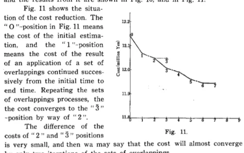
The overlapping method can be very easily applied to this process, and the results from it are shown in Fig. ID, and in Fig. 11.

Fig. 11 shows the situa-tion of the cost reducsitua-tion. The "0 "-position in Fig. 11 means the cost of the initial estima-tion, and the "1 "-position means the cost of the result of an application of a set of overlappings continued succes-sively from the initial time to end time. Repeating the sets of overlappings processes, the the cost converges to the

"3"

12.2 ~ 12.1

~

's ~ 12.0 U 11. o

-position by way of "2". 11·!S,\-o--t---Ir----.r--t----fo---Ir--Ir--+---->.

The difference of the

costs of " 2 " and"

3"

positions Fig. 11.

is very small, and then wa may say that the cost will almost converge by only two iterations of the sets of overlappings.

Therefore, if we start from the" 2 "-position using the average

CdF/dG)

Ct)

calculated at" 2 "-position and LlG=lO MW, the cost

dec-reases to the" 3 "-position by an application of the overlapping method. Repeating one more set of overlappings, the cost further reduces to "4". Again, CdFjdG) Ct) is recalculated at there, and so on.

Example Il.

(14)

structures: [ ; A ].

[:~~]~[:~]

BB A Xa ba C

c c ·

b4 (9)

For example, these are the bottle-neck problems, the expanding instal-lation system problems, etc. A, B, C are matrices, and we suppose the elements of each row of C have the same signs. Then, if we introduce the variables SI, S2, S3, St', S2', Sa',

SI=AXl S2=BXl+AX2 Sa=BXl+BX2+AXa St'=CtXl S2' =CIXl

+-

C2X2 Sa' = Cl XI +-C2X2+-C3X3 , equations (9) are transformed into

(Xl SI_51' X2 52 52' j ~3 __ S3 53') / A - / C - / i 1 ~ b2 .B-A / A - / =0 / C - / =0 / ~ ba B-A 1 A - / =0 11 C _11, =0 ! I I ~ b 4 __ I (10) (11) (12)

We may suppose for example, (Xl, SI, 5/), (Xa, Sa, 53') are deci-:sions, and (X2, 52, S2') are states, when we wish to deal with this pro-blem as a multi-stage decision process. (Formally, we may introduce (Xo

=0, So=O, 50'=0) as the states.)

When we wish to deal with this problem by the relaxation method _already decsribed in paragraph 3 (an extension of the multi-stage deci-.sion process), we may make eXI, SI, St'), (X2, S2, S2') and eX a, Sa, Sa'),

(15)

the I-stage variables, the I1-stage variables and the Ill-stage variables, and we may use the two kinds of the multi-stage decision processes

alternately.

7. BASIC CONCEPTS OF THE METHOD AND POSSIBILITIES OF THEIR EXTENSIONS.

The multi-stage decision problem described in paragraph 2 can be reduced to a problem which includes only the decisions X!, X2 , . " , or a problem which includes only the states SI, S2,"', if So are given.

It may appear that the treatment of a dynamic problem by a multi-stage decision process is wasteful from a standpoint of reducing the size of the over-all problem.

However, it is true that the method of subdivision can be accom-plished easily by the additions of the superfluous variables. We shall say as follows:

A matrix of a dynamic problem can be a matrix which has the stronger couplings between the stages, or can be a matrix which has the more loose couplings between the stages, according to the expres-sion of the problem.

To make the matrix, loosely coupled is accomplished by the addi-tions of the variables to the given system. This corresponds to expres-sing the inner structure more finely. On the other hand, a compact matrix expression of the system without the additional variables corre-sponds to the standpoint of viewing its structure from the outside, or of regarding the system as a black box, if we make an extreme argu-ment.

This basic concept will be included in the G. Kron's "Dia-koptics ". (6)

The other basic concept of the method is to observe that the dynamic problem consists of the many static problems having nearly the same structures. On account of it, we can deal with each sub-divided static problem on a common base, and the computations become very easy. (parametric programming).

One of the extensions of these basic concepts is a possibility of "Network Programming", and the other extension is a possibility of the easier computations by the refinement of the system.

(16)

ACKNOWLEDGEMENTS.

I am very much thankful to all the members of Dynamic Program-ming group of JUSE, for their kind discussions.

REFERENCES:

1) R. Bellman: Dynamic Programming, 1958.

2) G. B. Danzig: On the status of multi-stage linear program-ming problems, The RAND Corporation, p. 1028, 1957.

3) G. B. Danzig: Recent advances in linear programming, Management Science, Vo!. 2 .. No. 2, Jan. 1956.

4) G. B. Danzig: Upper bounds, secondary constraints, and block triangularity in linear programming, Econometrica, Vo!. 23, No. 2, April, 1955.

5) T. Fukao, T. Yamazaki: A computational method of economic operation of hydro-thermal power systems including flow-inter-connected hydro-plants, the Journal of I. E. E. of Japan, Vo!. 79, No. 5, May, 1959.

6) G. Kron: A set of principles to interconnect the solutions of physical systems, Journal of Applied Physics, vo!. 24, No. 8, August, 1953.