ROBUST ANALYSIS OF BOUNDARY SHAPE IDENTIFICATION ARISING IN THERMAL TOMOGRAPHY

(1)

ROBUST ANALYSIS OF BOUNDARY SHAPE IDENTIFICATION

ARISING IN THERMAL TOMOGRAPHY

Fumio Kojima

Mechanical Engineering Department Osaka Institute ofTechnology

5-16-1, Ohmiya, Asahi-ku, Osaka 535 JAPAN

Abstract: This paper is

concerned

with a choice ofregularization parameter for output least square identificationsofdistributed parameter systems. A method for adjusting the “optimal” regularization parameter isproposed basedonthegraphicalapproach. The idea

is applied to a geometrical heat inverse problem arising in thermal testing of materials. The effectiveness and validity of the method proposed are shown in both computational experiments and experiments with laboratory data.

1. INTRODUCTION

The output least square identification (OLSI) is a fundamental technique for solving

inverse problems. The method has been applied to various kinds of engineering problems

including oil exploration surveys, oil recoveries, computed impedance tomographies, etc.

The essential difficulties in engineering applications of OLSI come from the fact that real data are heavily corrupted by observation noise and it oftenoccurs that the corresponding

model output data are far from those practical data. This means most practical inverse

problems exhibit alack of continuous dependence of the estimated parameters on the data. Tikhonov regularization is one possible technique for avoiding these serious difficulties in computational efforts. Let $B$ be a parameter space and $C$ be the compact admissible

subset of $B$. The data space is denoted by $F$. Let $\phi$ be a continuous mapping from $C$

into $F$. Then the OLSI problem is to seek the minimum solution $\hat{q}\in C$ofthe fit to data

function

$J(q)= \frac{1}{2}||\phi(q)-y_{d}||_{F}^{2}$

.

(1)

Tikhonov’s method is to replace the cost (1) by one well-behaved regularized function

$J_{\eta}(q)=J(q)+ \frac{\eta}{2}||q-q_{0}||_{E}^{2}$ (2)

where $||\cdot||_{E}$ is the norm (or semi-norm) defined in $B$ and where $q_{0}$ denotes a priori

esti-mate of$q$. It is well-known that the above method ensures the robustness with respect to

perturbation of the data$y_{d}$. .This paper is concerned with the choice of regularization

pa-rameter $\eta$. In Section 2, the graphical method is introduced for the choice ofregularization

parameter. In Section 3, this scheme is applied to boundary estimation problems arising

in thermaltomography. In Section 4, the validity of the proposed method is demonstrated

through computational experiments. Finally, the method is applied to laboratory data

(2)

2. TIKHONOV REGULARIZATION

To solve the minimization problem of OLSI by regularization is now a fundamental

techniquefor parameter estimation problems. Tikhonov regularization ensures interesting

properties of the OLSI problem, such as existence of a minimum, stability with respect to perturbation of the data $y_{d}$. Let $\hat{q}(\eta)\in C$ be a solution of

$J_{\eta}( \hat{q}(\eta))=\min_{q\in C}J_{\eta}(q)$ (3)

such that

$\lim_{\etaarrow 0}\hat{q}(\eta)=\hat{q}(0)$. (4)

Tikhonov showed that there exists a constant $\gamma_{0}\in[0,\overline{\gamma}]$ such that,

for all $\delta>0$,

$||\phi(q_{0})-y_{d}||_{F}\leq M\sqrt{\eta}\leq\gamma_{0}$ $\Rightarrow$ $||\hat{q}(\eta)-q_{0}||_{E}\leq\delta$. (5)

This result givesus a useful insight on the choice ofregularization parameter $\eta$. Miller [2]

suggested

that the constant $M$ is set as an a priori upper bound on the parameter error

$\delta$. This means the regularization parameter can be chosen as

$\eta=(\frac{\gamma_{0}}{M})^{2}(or=(\frac{\gamma_{0}}{\sigma})^{2})$ . (6)

The crucial point of this method is to require an a prio$\prime ri$ upper bound on the measurement

error. Tikhonov and Arsenine [1] proposed another useful choice that was often called (Morozov principle”:

Given the upper bound of measurement error

$||\phi(q_{0})-y_{d}||_{F}\leq\gamma$, (7)

choose the regularization parameter $\eta$ in such a way that the residual norm is

equal to

$||\phi(\hat{q}(\eta))-y_{d}||_{F}=\gamma$. (8)

Although this method requires more computational efforts rather than Miller’s method,

no a priori upper bound $M$ is necessary. Adjustment can be done only by trials and

errors. Moreover, Kravaris and Seinfeld [3] showed the following asymptotic behavior:

$||\hat{q}(\eta(\gamma))-q_{0}||_{E}$ $arrow 0$ as $||\phi(q_{0})-y_{d}||_{F}\leq\gammaarrow 0$. (9)

This approach has been applied to many practical optimization algorithms. However, the

range of regularization parameter $\eta^{o}$ satisfying the above statement sometimes becomes

too large, so that, in practical applications, there are many cases where the feasible

regularization parameter $\eta(\gamma)^{o}$ could not determined by computational efforts. In other

words, the (optimal’ parameter $\eta^{o}$ must be chosen over $\eta(\gamma)\in\Theta$ where $\Theta$denotes the set

satisfying the above statement. One possible method forfindingthe optimal parameter $\eta^{o}$

is agraphical approach by means of L-curve. The outline of this approach is summarized

(3)

Fig. 1. Experimental set-up ofthermal testing ofmaterials Given $\eta$, solve

$J_{\eta}( \hat{q}(\eta))=\min_{q}J_{\eta}(q)$, (10)

for $\eta\in[0, \infty$), collect the points

$(||\phi(\hat{q}(\eta))-y_{d}||_{F}, ||\hat{q}(\eta)||_{E})$ (11)

and plot the above points. Then the “optimal” parameter $\eta^{o}$ can be chosen

as apoint that lies in the “corner” ofthe resulting

curve.

Existence of such “L”-shapedcurve was well-known for the ill-posed algebraiclinear

prob-lems, such

as

the discrete solver of integral equation of the first kind. Recently, Hansen [4] overviewed this graphical approach for the discrete ill-posed linear problems. More

careful discussions have been done by Kitagawa [5]. The plotting curve was first named

(

$L$’-curve by Hansen in his

paper’.

Our attempt is to use this method for the nonlinear

least square problems.

3. THERMAL TESTING OF MATERIALS

In this section, the methodis applied

to

a geometrical heat inverse problem arisingin thermal testing of materials. The problemis motivatedbythe

non-destructive

evaluation in aerospace structures. The overall configulation ofthe evaluation system is illustrated

in Fig. 1. As shown in Fig. 1, the problem is to estimate the backsurface corrosion shape using the thermographical data from the front surface. The corresponding inverse

problem is formulated as a parameter estimation problem. We restrict our attention in

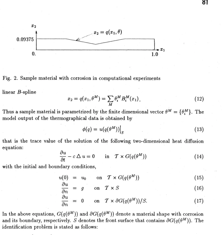
estimating the shape of backsurface in Fig. 2. The corrosion shape is approximated by

(4)

Fig. 2. Sample material with corrosion in computational experiments linear B-spline

$x_{2}=q(x_{1}, \theta^{M})=\sum_{AI}\theta_{j}^{M}B_{t}^{M}(x_{1})$

.

(12)

Thus a sample material is parametrized by the finitedimensional vector $\theta^{M}=\{\theta_{i}^{M}\}$. The

model output of the thermographical data is obtained by

$\phi(q)=u(q(\theta^{M}))|_{S}$ (13)

that is the trace value of the solution of the following two-dimensional heat diffusion

equation:

$\frac{\partial u}{\partial t}-c\triangle u=0$ in $\mathcal{T}\cross G(q(\theta^{M}))$ (14)

with the initial and boundary conditions,

$u(0)$ $=$ $u_{0}$ on $\mathcal{T}xG(q(\theta^{Af}))$ (15)

$\frac{\partial u}{\partial n}$

$=$ $g$ on $\mathcal{T}\cross S$ (16)

$\frac{\partial u}{\partial n}$

$=$ $0$ on $\mathcal{T}\cross\partial G(q(\theta^{M}))/S$. (17)

In the above equations, $G(q(\theta^{M}))$ and $\partial G(q(\theta^{M}))$ denote a material shape with corrosion

and its boundary, respectively. $S$denotes the front surface that contains $\partial G(q(\theta^{M}))$. The

identification problem is stated as follows:

Given $\{u_{0}, g, y_{d}\}$, determine geometrical structure of the sample material, in

other words, estimate $\theta^{M}$

.

The computational techniques we have employed is based on the use of a finite element

Galerkin approach to construct a sequence of finite dimensional approximating

identi-fication problems. Let us choose $\bigcup_{N}\{B_{t}^{N}\}$ as a set of basis functions in _$H^{1}(C)$ and

approximate the finite Galerkin solution of (14) by

$u^{N}(t, q)= \sum_{N}w^{N}(t, q)B^{N}$

.

(18)

Then the coefficient

vector

$w^{N}(t, q)=\{w_{i}^{N}\}$ yields linear systems of equations:

(5)

with

$w^{N}(0, q)=\overline{w}_{0}^{N}(q)$. (20)

The computational method for the identification problem is given by (IDP) Find $\hat{\theta}^{M,N}$

which minimizes

$J_{\eta}^{M,N}( \theta^{M})=\frac{1}{2}\Vert\phi^{M,N}(q)-y_{d})\Vert_{F}^{2}+\frac{\eta}{2}\Vert q(\theta^{M})\Vert_{E}^{2}$ (21)

subject to

$\phi^{M,N}(q)=\sum_{N}w^{N}(t, q(\theta^{M}))B^{N}|_{S}$

.

(22)

and the linear ordinary

differential

equation (19) with (20).

The purpose of this regularization is to smooth the estimated curve related to corrosion

shape. The stabilization ofdifferentialcomponents of the estimatedcurveplayanessential role in this smoothing. Taking int$0$ account this, the semi-norm of $H^{1}(0,1)$ is taken as

the regularization term:

$\Vert q(\theta^{M})\Vert_{E}^{2}=\Vert\frac{dq}{dx_{1}}(\theta^{M})\Vert_{L^{2}(0,1)}^{2}=\sum_{i}|\theta_{i}^{M}-\theta_{i-1}^{M}|^{2}$ (23)

4. COMPUTATIONAL EXPERIMENTS

In our computational experiments, a corrosion shape is assumed to be a steel sample with damage as depicted in Fig. 2. A sample was assumed with dimensions $0.09375\cross$

1. inch. A test example is constructed as follows. A true parameter vector $\theta_{o}^{M}$ in (12)

is given. The corresponding solution is computed by solving (19). Simulated data are generated by adding random noise to the numerical solution of (19):

$y_{d}=\phi^{M,N}(q(\theta_{o}^{M}))+\epsilon$ (24)

where $\epsilon$ implies additive disturbance given by Gaussian randomsequence with $N(0. , \sigma^{2})$.

In this procedure, the dimensions of the unknown parameter vectors were taken as

$dim(\theta^{M})=7$

.

The value of the true parameters were chosen as

$\theta_{O}^{M}$ _$=$ [0.08203125,0.0703125,0.05859375,0.46875,

0.05859375,0.0703125, 0.08203125].

The number of nodes related to finite elements in the computational experiments were set as $N=165$. The estimated sequence $\hat{\theta}^{M}$

was computed by using the optimization routine for nonlinear least square problems. The trust region method is adopted to the problem (IDP). For the implementation of the trust region algorithm, a Fortran software

(6)

$\infty\Phi$

B..

$\frac{os}{B}$ $\sigma_{\not\subset}^{(o}Q$ $\overline{\neg 9)}$ $\frac{9Nc\dotplus}{o}D$ $(arrow S^{0}\neg$ $\overline{\overline{\underline{\aleph\sigma}cb^{Q}\cdot}}$ $\overline{\Phi\leq}$ $\overline{\overline{\triangleright_{\grave{\omega}}}}-$ \={o} $–$

Residual

norm

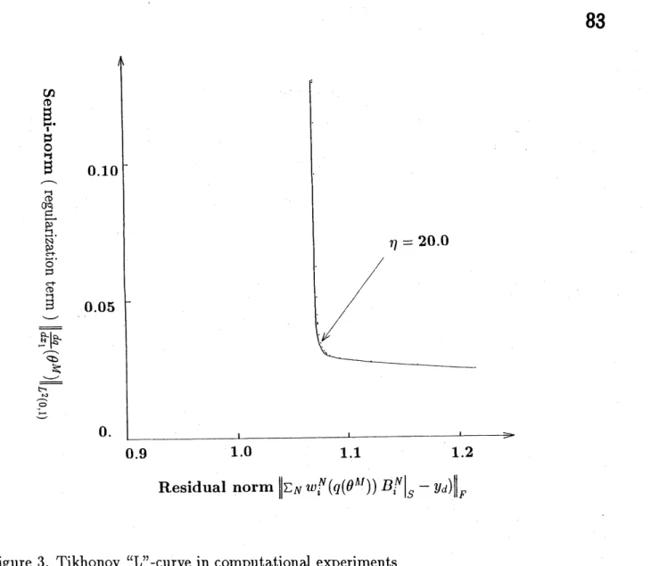
$\Vert\Sigma_{N}w_{i}^{N}(q(\theta^{AI}))B_{i}^{N}|_{S}-y_{d})\Vert_{F}$

Figure 3. Tikhonov $L$’-curve in computational experiments

this computational experiments is to confirm the existence of distinct “corner” drawing the curve,

(

$\Vert\sum_{N}w_{i}^{N}(q(\theta^{M}))B_{i}^{N}|_{S}-y_{d}\Vert_{F}$, $\Vert\frac{dq}{dx_{1}}(\theta^{M})\Vert_{L^{2}(0,1)}$

).

To this end, for each $\eta\in[0, \infty$), the optimization problem (IDP) was solved numerically

and the value of residual norm $\Vert\Sigma_{N}w_{i}^{N}(q(\theta^{M}))B_{i}^{N}|_{S}-y_{d})\Vert_{F}$ and the semi-norm

(reg-ularization term) $\Vert\frac{d}{dx}L_{1}(\theta^{M})\Vert_{L^{2}(0,1)}$ were computed. Figure 3 depicts the corresponding

“L”-curve for the data with the random noise $\sigma=0.2$. The results illustrates that the

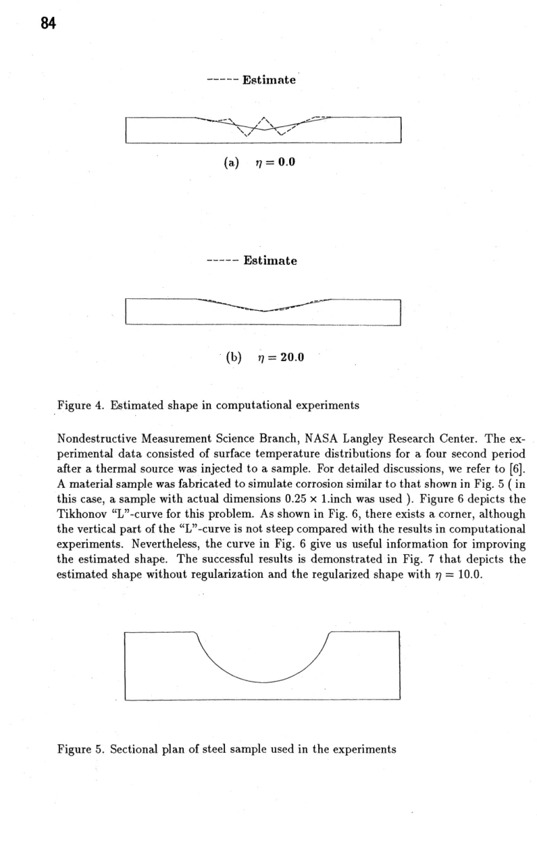
curve has a distinct corner around a point corresponding to $\eta=20$. Figure 4 shows the

estimated shape without regularization and the regularized shape with $\eta=20$.

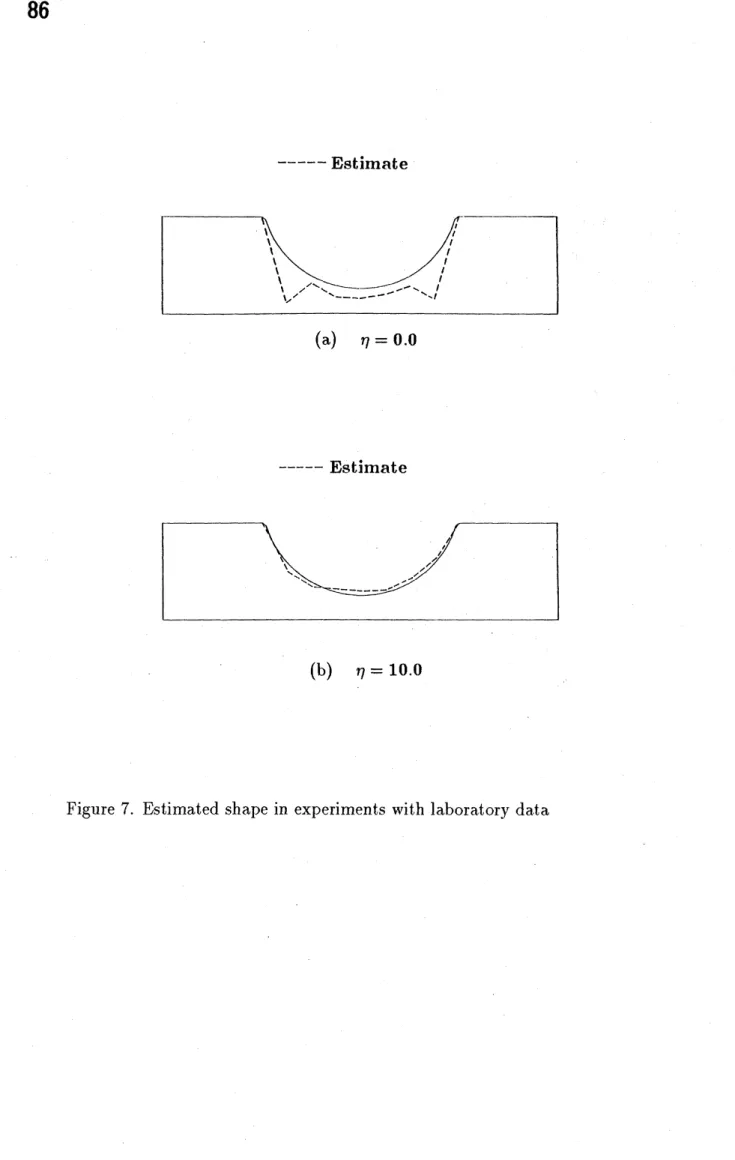
5. EXPERIMENTS WITH LABORATORY DATA

In this section, the results of using our estimation procedures are reported with ex-perimental data. All experiments were carried out in the Instrument Research Divisions,

(7)

$—-$

_-Estimate

–\sim $J^{\wedge}\backslash _{\backslash }$

$\nearrow^{\prime-}$

$\backslash _{\backslash }/$ $\backslash /’$

’

(a) $\eta=0.0$

$—-$

-Estimate

(b) $\eta=20.0$

Figure 4. Estimated shape in computational experiments

Nondestructive Measurement Science Branch, NASA Langley Research Center. The

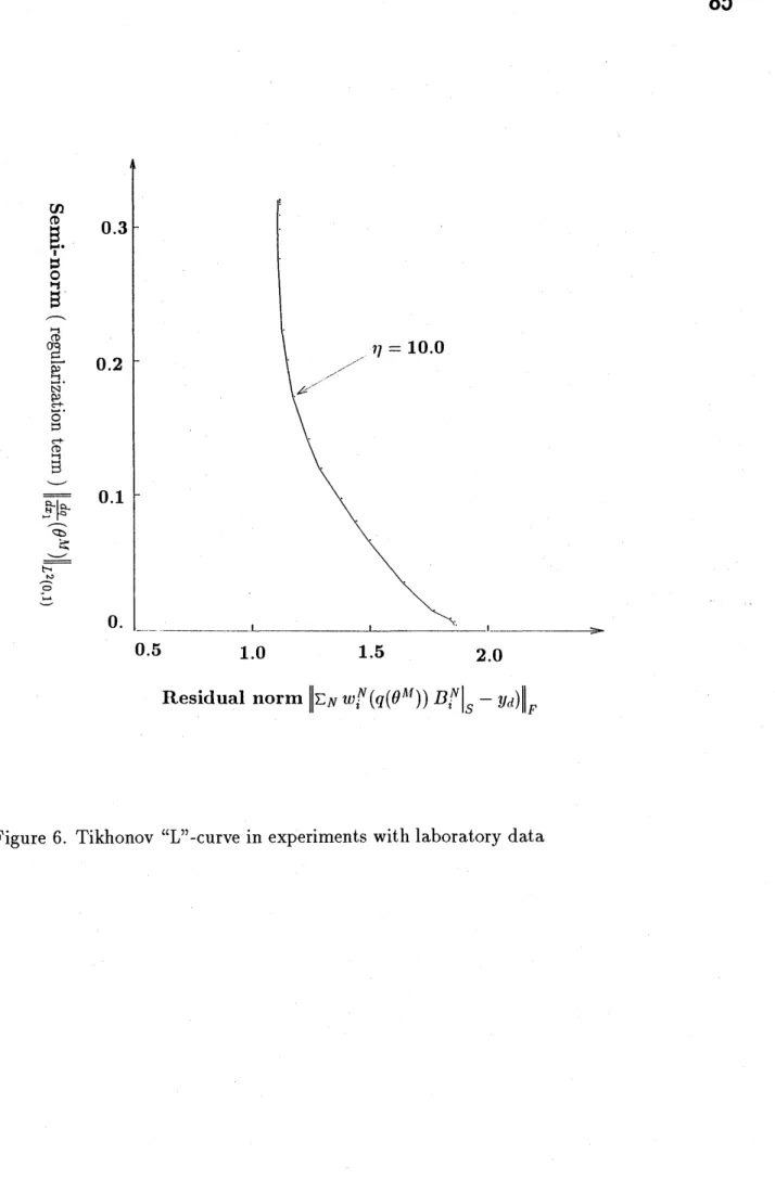
ex-perimental data consisted of surface temperature distributions for a four second period after a thermal source was injected to a sample. For detailed discussions, we refer to [6]. A material sample wasfabricated to simulate corrosion similar to that shown in Fig. 5 (in this case, a sample with actual dimensions 0.25 $x$ l.inch was used). Figure 6 depicts the

Tikhonov $L$’-curve for this problem. As shown in Fig. 6, there exists a corner, although

the vertical part of the (_$L’$

-curve is not steep compared with the results in computational

experiments. Nevertheless, the curve in Fig. 6 give us useful information for

improving

the estimated shape. The successful results is demonstrated in Fig. 7 that depicts the

estimated shape without regularization and the regularized shape with $\eta=10.0$.

(8)

$\infty\Phi$ $B_{l}.$

.

$s\frac{o}{B}$ $\sigma_{\frac{\neg\Phi\not\in}{\underline{g}}}$ . $N\frac{g}{s\circ}$. $B\neg co\epsilon+$ $\overline{\overline{tL\underline{rightarrow}b^{a}\cdot}}$ $\overline{\Phi}$ $\nwarrow$ $\overline{\overline{h^{-}}}$ \={o} $\underline{-}$ 0.5 1.0 1.5 _2.0

Residual norm$\Vert\dagger r$

Figure 6. Tikhonov ((_$L’$

(9)

$—–$ Estimate

(a) $\eta=0.0$

$—-$ Estimate

$\backslash _{\backslash }\backslash \backslash _{\backslash }$

$-_{---\prime}’\prime^{P^{\prime^{\prime’}}}/’$

’

(b) $\eta=10.0$

(10)

6. CONCLUDING REMARKS

A graphical method was proposed for determiningthe (optimal’ Tikhonov parameter

by using L-curve. The proposed scheme is quite simple, easy to apply and no a priori

statistical information is necessary. For each computational experiment with a different

noise level, it was shown that L-curve yields a “distinct” corner on the residual versus the

semi-norm $pIane$, so that the “optimal” regularization parameter could be easily chosen.

Although there are many open problems on the theoretical part of this approach, the validity and applicability of the proposed method were demonstrated through the use of both the computational and laboratory data.

ACKNOWLEDGEMENTS

This research was carried out in part while the author was a visiting scientist at the

Institute for Computer Applications in Science and Engineering (ICASE), NASA Langley

Research Center, Hampton, Virginia, VA 23665 during August 1991. The author would

like tothank Professor H.T. Banks for his encouragement topursue this research. Thanks

are also extended to Dr. W.P. Winfree at Nondestructive

Measurement

Science Branch,

NASA Langley Research Center for providing the thermal data and to Dr. R.G. Carter

for his helpful discussions on the use of the optimization algorithm.

References

[1] A. Tikhonov and V. Arsenine, Solutions of Ill-posed Problems, John-Wiley, 1977.

[2] K. Miller, “Least-squares methods for ill-posed problems with a prescribed bound,” SIAM J. Math. Anal., Vol. 1 (1970).

[3] C. Kravaris and J.H. Seinfeld, $\zeta Identification$ of parameters in distributed

parame-ter systems by regularization,” SIAM J. Control and optimization, Vol. 23 (1985)

pp. 217-241.

[4] P.C. Hansen, ((

$Analysis$ of discrete ill-posed problems by means of the L-curve,”

Submitted to SIAM Rev..

[5] Kitagawa, “Optimal regularization for ill-posed problems by means ofL-curve,” this

lecture notes.

[6] H.T. Banks, F. Kojima, and W.P. Winfree, (Boundary estimation problems arising

in thermal tomography,” ICASE Report No. 89-44, NASA Langley Research Center: Inverse Problems, Vol. 6 (1990) pp. 897-921.

[7] R.G. Carter, ‘Safeguarding Hessian approximations in trust region algorithms,”

Technical Report TR-87-12, Department of Mathematical Sciences, Rice University,