journal or
publication title
KGPS review:Kwansei Gakuin policy studies
review
number
25
page range
15-32
year
2018-03-31
15
Does Financial Risk Explain Japan’s Great Stagnation?
Ayato ASHIHARA
1【修士論文概要書】
Abstract:
Japan has experienced a long-lasting stagnation since the early 1990s. According to the Reference Dates of Business Cycle, the Cabinet Office of Japan, there are four recession periods between 1987 and 2010, and three of them are considered to be financially-related. This implies that the stagnation was triggered by financial factors. Nonetheless, many studies using Dynamic Stochastic General Equilibrium models claim that a decline in Total Factor Productivity is the main driver of the stagnation. To resolve this contradiction, this study estimates the Japanese economy by a New-Keynesian DSGE model augmented with financial friction used in Christiano, Motto and Rostagno (2014), where “risk shock” is newly incorporated into the model that refers to uncertainty in the financial market. According to our estimation results, the estimated risk shock can explain the overall fluctuations of GDP and investment, and thus it is considered to be the main driver of the stagnation. We also find that it is highly correlated with the Business condition Diffusion Index, the Financial Position Diffusion Index and the Lending Attitude Index of Financial Institutions in Tankan released by the Bank of Japan. Therefore, we conclude that the estimated risk shock can be interpreted as the firms’ distrust toward their business conditions, and it delayed their investment decisions, then causing the prolonged economic contraction.
Key words and Phrases: Japan’s Great Stagnation in the 1990s, Risk shock, Estimated DSGE models
1. Background and Motivation
Japan has experienced a long-lasting stagnation since the early 1990s. During this period, the average growth rate was down to 1.1%, compared to 4.4% in the 1980s. Figure 1 plots its real GDP growth rate from 1987 to 2010. The impacts on the Japanese society was enormous. Deterioration of the employment environment is one example of these. According to Recruit Works Institute, the effective job offer rate for university graduates started to decline from 1990, and eventually went below unity in 2000. To avoid the same circumstance in the future, it is desirable to consider what it was that brought this stagnation.
According to the Reference Dates of Business Cycle, the Cabinet Office of Japan, there are four
16
recession periods, which are shown as the shaded areas in Figure 1. In particular, three of them are related to financial crisis. The first was due to the corruption of asset price bubbles in the early 1990s. Prices of stock and real estate, which had risen from middle-1980s, dropped sharply, and this affected the real economy through the negative wealth effect and malfunction of financial intermediation (Bayoumi, 2001). The second recession, which happened in the late 1990s, stemmed from the successive bankruptcies of financial institutions that had suffered from the impairment of their balance sheets after the former recession. The confusion in the inter-bank market due to the default of Sanyo Securities triggered a considerable number of bankruptcies of financial institutions, such as Hokkaido-Takushoku bank and Yamaichi securities, and many literatures including Motonishi and Yoshikawa (1999) mention that this crisis influenced the real economy through the credit crunch channel. The third was what is called the Great Recession. Although it originated in U.S., the spillover effect decreased exports from Japan. Considering these episodes, Japan’s Great Stagnation is considered to be caused by financial factors. However, the previous literature using DSGE model points out a decline in TFP, or neutral technology, as the main factor (the detail explained later).
2. Previous Studies
Since the asset bubble burst in the early 1990s, a considerable number of studies about Japan’s Great Stagnation have been conducted. Hayashi and Prescott (2002), a pioneering study, refer to the decline in TFP and the reduction of workweek length from 44 to 40 hours as the main causes in a RBC model framework. On the other hand, Christiano and Fujiwara (2006), using a standard DSGE model with “news shock”, suggest that the combination of Pigue effect and reduction of workweek length can also replicate
the stagnation.2 They also suggest the importance of incorporating Investment Specific Technological
(IST) shock because the relative price of investment had continuously fallen for ten years from 1990. Hirose and Kurozumi (2012) incorporate the IST shock into an otherwise standard DSGE model and obtain the similar results to Hayashi and Prescott (2002). They also find that Marginal Efficiency of Investment shock
(hereafter M.E.I. shock) is more important than the IST shock for investment fluctuation.3 According to
Justiniano, Primiceri and Tambalotii (2011), the M.E.I shock is related to financial factors, and thus Kaihatsu and Kurozumi (2014) use a standard new Keynesian model embodied with Financial Accelerator of BGG and find similar results to Hayashi and Prescotti (2002). They also find a high correlation between the dynamics of the neutral technology shock and the diffusion index of firms’ financial position in Tankan and conclude that the tight financing position decreased R&D investment, and thus neutral technology.
2 While Christiano and Fujiwara (2006) calibrate structural deep parameters of the model, Fujiwara, Hirose and
Shintani (2008) estimate the parameters by the Smets and Wouters (2003, 2007) method. They conclude that news shock in TFP largely accounts for the fluctuation of the Japan’s Great Stagnation.
3 Sugo and Ueda (2008) use a New-Keynesian model similar to those of Christiano, Eichenbaum and Evans (2005),
17
Almost all studies using DSGE model refer to the TFP shock as the main factor of Japan’s Great
Stagnation.4 However, these studies have some problems. First, five studies do not incorporate financial
frictions into their model. As explained above, financial friction is the essential factor for analyzing Japan’s Great Stagnation. Second, Kaihatsu and Kurozumi (2014)’s result implies rather the tight firms’ financial position as the main driver rather than the decline in TFP. The reason why TFP shock becomes the main factor may be that the financial shocks used in their model fail to express actual business cycles we can observe in data. In fact, CMR (2014), using the model embodied with “risk shock” in addition to standard shocks, suggest that canonical financial shocks cannot replicate the U.S. business cycle. They also find that the estimated risk shock accounts for 62% of GDP and 73% of investment. Therefore, in this paper, we reconsider Japan’s Great Stagnation by using their model.
3. The model
DSGE model is a kind of macroeconomic models, which considers dynamic optimal behaviors of economic agents (such as household and firm) explicitly. It is mainly used for the factor analysis of business cycles. It can be expressed as a linear state space model when its equations are log-linearized and then solved under the assumption of rational expectation, for example Blanchard and Khan (1980) and Sims (2002). Namely, formularizing both its optimization equations and constraint equations as simultaneous differential equations, considering predetermined variables in the model as state variables in transition equation of the state space model and adding observation equations which connect state variables to observed variables, we can express DSGE model as such a way. Therefore, Bayesian estimation methods with MCMC method are often used for the DSGE estimation.
Smets and Wouters (2003, 2007) is a pioneering study which estimates a standard New-Keynesian DSGE model in this way. They estimate Europe and U.S. economies and conclude that the model fits to the data enough to bear comparison with vector autoregressive models whose model restriction is weaker than that of DSGE. Now, many researches using this method are conducted all over the world.
The model we use is CMR (2014). This model has six frictions to fit the data; both nominal price and wage stickiness, adjustment costs of investment and capital utilization, asymmetric information (between lender and borrower) and Costly State Verification (CSV, hereafter) which is originally analyzed in Townsend (1978). The combination of last two frictions is so-called Financial Accelerator developed by BGG (1999). It enables us to incorporate a channel through a financial crisis into the business cycle analysis. There are 7 agents in the model; the final goods producer, intermediate goods producers, entrepreneurs, the mutual fund, the household, the wage contractor and the government.
4 The exception is Hirakata, Sudo, Takei and Ueda (2014). They use a canonical New-Keynesian model with the
18
We briefly explain the setting of financial market, which is deeply concerned with risk shock.5 For
simplicity, we focus on the essence of financial market mechanism, so the explanation is not strict. There
exist entrepreneurs and mutual fund. Entrepreneurs combine their net worth 𝑁𝑁 and borrowings 𝐵𝐵𝑡𝑡+1𝑁𝑁
from the mutual fund (its ultimate source is household), and purchase raw capital 𝐾𝐾𝑡𝑡+1𝑁𝑁 (ex. iron, steel,
plastic, etc.). They transform it into effective capital and sell it to household.
𝐾𝐾𝑡𝑡+1𝑁𝑁 = 𝑁𝑁 + 𝐵𝐵𝑡𝑡+1𝑁𝑁 (1.1)
After capital purchase, entrepreneurs receive an idiosyncratic shock 𝜔𝜔, and the raw capital converts into
effective capital 𝜔𝜔𝐾𝐾𝑡𝑡+1𝑁𝑁 , 𝜔𝜔~𝐹𝐹(1, 𝜎𝜎𝑡𝑡). 𝐹𝐹(∙) is a log-normal cumulative function. 𝜎𝜎𝑡𝑡 is standard deviation
of 𝜔𝜔 and follows AR(1) process. We call this risk shock because it captures uncertainty about the future
success of their products. Entrepreneurs rent effective capital to firms at rental rate 𝑟𝑟𝑡𝑡+1 in 𝑡𝑡 + 1. After
firms’ production, they sell undepreciated capital 𝜔𝜔𝐾𝐾𝑡𝑡+1𝑁𝑁 (1 − 𝛿𝛿) . 𝛿𝛿 is depreciation rate. Total capital return rate is 𝜔𝜔(1 + 𝑅𝑅𝑡𝑡+1𝐾𝐾 ) where 1 + 𝑅𝑅𝑡𝑡+1𝐾𝐾 ≡ 𝑟𝑟𝑡𝑡+1+ 1 − 𝛿𝛿 is a constant rate of return project. New
worth of an entrepreneur with net worth 𝑁𝑁 in 𝑡𝑡 + 1 and who experiences shock 𝜔𝜔 is
𝑁𝑁′= max{0, (1 + 𝑅𝑅
𝑡𝑡+1 𝐾𝐾 )𝐾𝐾
𝑡𝑡+1𝑁𝑁 𝜔𝜔 − 𝑍𝑍𝑡𝑡+1𝐵𝐵𝑡𝑡+1𝑁𝑁 }. (1.2)
where 𝑍𝑍𝑡𝑡+1 is gross rate of interest on loan. The banking system in period 𝑡𝑡 is competitive. The following
zero profit condition must be satisfied.
𝐿𝐿𝑡𝑡≡𝐾𝐾𝑡𝑡+1 𝑁𝑁 𝑁𝑁 = 1 1 − 1 + 𝑅𝑅𝑡𝑡+1𝐾𝐾 1 + 𝑅𝑅𝑡𝑡 [𝛤𝛤(𝜔𝜔�𝑡𝑡+1, 𝜎𝜎𝑡𝑡) − 𝜇𝜇𝜇𝜇(𝜔𝜔�𝑡𝑡+1, 𝜎𝜎𝑡𝑡)] (1.3) Γ𝑡𝑡(𝜔𝜔�𝑡𝑡+1, 𝜎𝜎𝑡𝑡) ≡ [1 − 𝐹𝐹𝑡𝑡(𝜔𝜔�𝑡𝑡+1, 𝜎𝜎𝑡𝑡)]𝜔𝜔�𝑡𝑡+1+ 𝜇𝜇𝑡𝑡(𝜔𝜔�𝑡𝑡+1, 𝜎𝜎𝑡𝑡), 𝜇𝜇𝑡𝑡(𝜔𝜔�𝑡𝑡+1, 𝜎𝜎𝑡𝑡) = � 𝜔𝜔𝜔𝜔𝐹𝐹𝑡𝑡(𝜔𝜔, 𝜎𝜎𝑡𝑡) 𝜔𝜔�𝑡𝑡+1 0 ,
where 𝐿𝐿𝑡𝑡 is leverage. 𝜔𝜔�𝑡𝑡+1 is a cutoff value which divides entrepreneurs who can repay interest and
principle from those who cannot. The mutual fund audit entrepreneurs who receive 𝜔𝜔 ≤ 𝜔𝜔�𝑡𝑡+1 and get
back their all earnings. 𝜇𝜇 is a parameter of their monitoring cost. Therefore, 𝛤𝛤(𝜔𝜔�𝑡𝑡+1) − 𝜇𝜇𝜇𝜇(𝜔𝜔�𝑡𝑡+1) means the mutual fund’s share of average entrepreneurial earnings. Entrepreneurs select the borrowing contract at
period 𝑡𝑡 which maximizes the expected 𝑁𝑁′ subject to the zero profit condition and 𝑁𝑁. To increase their
profit, entrepreneurs select high leverage. However, the mutual fund rise interest on loan (or 𝜔𝜔�𝑡𝑡+1 )
according to the zero profit condition. Entrepreneurs’ first order condition with regard to 𝜔𝜔�𝑡𝑡+1 is
1 − 𝐹𝐹(𝜔𝜔�𝑡𝑡+1, 𝜎𝜎𝑡𝑡) 1 − 𝛤𝛤(𝜔𝜔�𝑡𝑡+1, 𝜎𝜎𝑡𝑡) = 1 + 𝑅𝑅𝑡𝑡+1𝐾𝐾 1 + 𝑅𝑅𝑡𝑡 [1 − 𝐹𝐹(𝜔𝜔�𝑡𝑡+1, 𝜎𝜎𝑡𝑡) − 𝜇𝜇𝜔𝜔�𝑡𝑡+1𝐹𝐹 ′(𝜔𝜔� 𝑡𝑡+1, 𝜎𝜎𝑡𝑡)] 1 − 1 + 𝑅𝑅𝑡𝑡+1𝐾𝐾 1 + 𝑅𝑅𝑡𝑡 [𝛤𝛤(𝜔𝜔�𝑡𝑡+1, 𝜎𝜎𝑡𝑡) − 𝜇𝜇𝜇𝜇(𝜔𝜔�𝑡𝑡+1, 𝜎𝜎𝑡𝑡)] . (1.4)
The left side of (1.4) means elasticity of entrepreneur’s expected return with regard to 𝜔𝜔�𝑡𝑡+1, and the right
side means elasticity of leverage with regard to 𝜔𝜔�𝑡𝑡+1. Given the cutoff, we can solve for leverage through
19
the zero profit condition (𝐾𝐾𝑡𝑡+1𝑁𝑁 is also determined). Risk shock 𝜎𝜎𝑡𝑡 deviates the shape of 𝐹𝐹(𝜔𝜔�𝑡𝑡+1, 𝜎𝜎𝑡𝑡). To satisfy the zero profit constraint, the mutual fund rise the cutoff value and interest on loan, which impedes capital accumulation.
4. Empirical methodology and results
Following Smets and Wouters (2003, 2007), the model presented in the previous section is estimated, using a Bayesian likelihood approach with twelve quarterly time series: output, consumption, investment, labor, real wage, inflation, relative price of investment goods, monetary policy rate, real loans, real net worth, price of stock and term premium. First, we estimate unobservable variables by the following linear state space model. The reason why we use the linear state space model is to estimate unobservable endogenous variables in the model whose corresponding data is difficult to find (ex. risk premium).
𝒚𝒚𝒕𝒕= 𝑨𝑨(𝜽𝜽) + 𝑩𝑩(𝜽𝜽)𝒔𝒔�𝒕𝒕, (2.1)
𝒔𝒔�𝒕𝒕= 𝚽𝚽𝟏𝟏(𝜽𝜽)𝒔𝒔�𝒕𝒕−𝟏𝟏+ 𝚽𝚽𝜺𝜺(𝜽𝜽)𝜺𝜺𝒕𝒕, (2.2)
where 𝒚𝒚𝒕𝒕 and 𝒔𝒔�𝒕𝒕 are vectors of observable variable (data) and unobservable variable (endogenous
variables in the model) respectively. 𝑨𝑨(𝜽𝜽) and 𝑩𝑩(𝜽𝜽) are vectors depend on structural deep parameters,
𝜽𝜽. 𝚽𝚽𝟏𝟏(𝜽𝜽) and 𝚽𝚽𝜺𝜺(𝜽𝜽) are coefficient matrixes, which are also dependent on 𝜽𝜽. 𝜺𝜺𝒕𝒕 denotes the aggregate
shock vector.
Second, we simultaneously estimate by the Bayesian Inference the structural deep parameters
necessary for the first estimation.6
Third, we conduct historical decomposition in order to detect the most influential aggregate shock on
the economy. Equation (2.2) can be rewritten so that unobservable endogenous variables, 𝒔𝒔�𝒕𝒕, is expressed
by its initial values, 𝒔𝒔�𝟏𝟏, and the sum of each aggregate shock, 𝜺𝜺𝒊𝒊, from period 1 to 𝑡𝑡. 𝒔𝒔�𝒕𝒕= 𝚽𝚽1𝑡𝑡−1(𝜽𝜽)𝒔𝒔�𝟏𝟏+ � 𝚽𝚽1𝑡𝑡−𝑖𝑖−1
𝒕𝒕−𝟏𝟏
𝒕𝒕=𝟏𝟏
(𝜽𝜽)𝚽𝚽𝜀𝜀(𝜽𝜽)𝜺𝜺𝒊𝒊+𝟏𝟏
Since the observation equations are 𝒚𝒚𝒕𝒕= 𝑨𝑨(𝜽𝜽) + 𝑩𝑩(𝜽𝜽)𝒔𝒔�𝒕𝒕, the fluctuation of 𝒚𝒚𝒕𝒕 can be decomposed by its
initial values, 𝒔𝒔�𝟏𝟏, and the cumulative sum of exogenous shocks, 𝜺𝜺𝒕𝒕, and we can observe the best shock that
replicate some selected variables of 𝒚𝒚𝒕𝒕.7 This is called the historical decomposition.
Equilibrium conditions and resource constraints are rewritten to be detrended since the model converges the balanced growth path in longer term, and these equations are log-linearized around deterministic steady states.
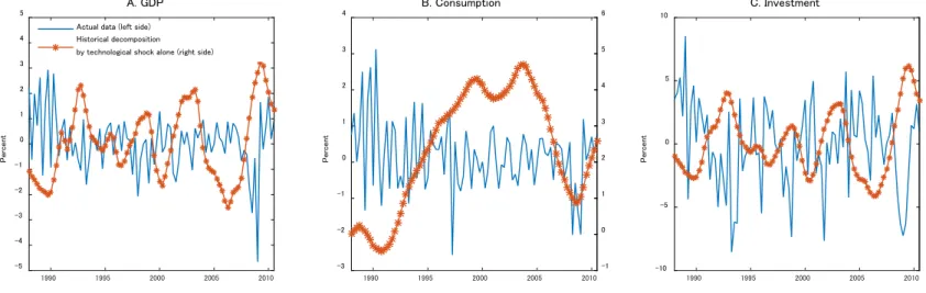
Figure 2 to 4 illustrate comparisons between time series of the selected data, GDP, consumption and investment, and those of corresponding endogenous variables calculated by historical decomposition of
6 For the detail discussion, see An and Schorfheide (2007). Parameter estimate results are shown in Appendix B.
20
three aggregate shocks and actual data, respectively. The lines with circle represent results of simulating model response to selected shocks and initial conditions. The solid lines are growth rates of the actual data.
The comparison between time series of the selected data and those of corresponding endogenous variables produced by a sum of the estimated persistent and transitory technological shocks is shown in Figure 2. It is difficult to mention that the two technology shocks can account for fluctuations of the actual data. Rather, the lines with circle of GDP and investment indicate the opposite behaviors to the solid lines (actual data).
Figure 3 shows the comparison between time series of the selected data and those of corresponding endogenous variables produced by the estimated marginal efficiency of investment (M.E.I) shock.The estimated M.E.I shock reproduces the opposite fluctuation to sharp drops in recessions. In particular, this is clearly found in investment. According to CMR (2014), M.E.I. shock represents supply shifter in the capital market. Therefore, the implication from this comparison is that the fall of investment throughout the stagnation does not stem from supply side in the capital market.
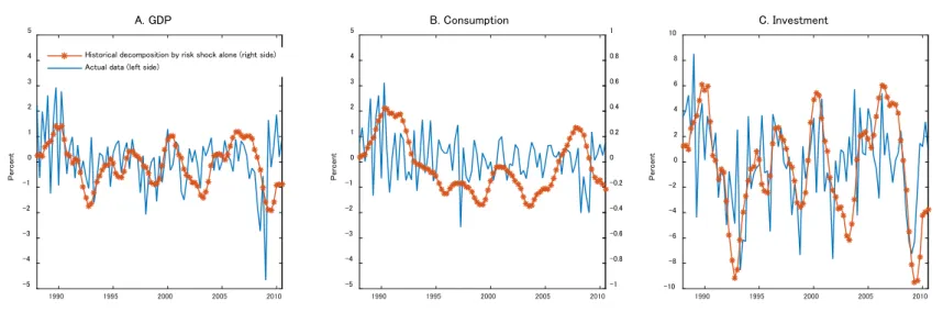
The comparison between time series of the selected data and those of corresponding endogenous variables produced by the estimated risk shock is shown in Figure 4. A remarkable feature in this figure is the closeness between the lines with circle and the solid lines. Above all, in terms of GDP and investment, explanations of the estimated risk shock are highly accurate from 1990:1Q to 2001:4Q which corresponds so-called “Lost Decade”. Therefore, this graph suggests that the estimated risk shock can largely account for the sharp falls of GDP and investment in recessions. Because the estimated risk shock represents demand shifter in the capital market, it is possible that the fall of investment during 1990s stems from the demand side in the capital market. In addition, the movement of actual consumption can be explained better by the estimated risk shock than by the other two estimated shocks. Therefore, it can be said that the estimated risk shock is more significant than the other shocks and the main driver of the Japan’s great stagnation.
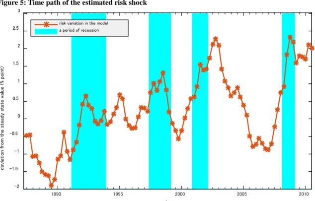
The historical decomposition clarifies the significance of “risk shock” in the Japan’s Great Stagnation. Then, it should be figured out what the estimated risk shock represents. This subsection analyzes the implication of the estimated risk shock from various perspectives.
To do this, we calculate the correlation coefficient between the estimated risk shock and various
measures: Diffusion Index for Business Condition, Financial Position and Lending Attitude in Tankan
released by the Bank of Japan (Table 4). It is highly correlated with the Business condition Diffusion Index, the Financial Position Diffusion Index and the Lending Attitude Index of Financial Institutions (Figure5). Therefore, we conclude that the estimated risk shock can be interpreted as the firms’ distrust toward their business conditions, and it delayed their investment decisions, then causing the prolonged economic contraction.
21
AppendixA: Complete model
Production function𝑌𝑌𝑗𝑗𝑡𝑡 = 𝜀𝜀𝑡𝑡𝐾𝐾𝑗𝑗𝑡𝑡𝛼𝛼�𝑧𝑧𝑡𝑡𝑙𝑙𝑗𝑗𝑡𝑡�1−𝛼𝛼− Φ𝑧𝑧𝑡𝑡∗ (A.1)
Optimal capital and labor input
𝑟𝑟𝑡𝑡𝑘𝑘= 𝛼𝛼𝜀𝜀𝑡𝑡�𝑧𝑧𝐾𝐾𝑡𝑡𝑙𝑙𝑗𝑗,𝑡𝑡 𝑗𝑗,𝑡𝑡� 1−𝛼𝛼 𝑠𝑠𝑡𝑡 (A.2) 𝑊𝑊𝑡𝑡= (1 − 𝛼𝛼)𝜀𝜀𝑡𝑡�𝑧𝑧𝐾𝐾𝑡𝑡𝑙𝑙𝑗𝑗,𝑡𝑡 𝑗𝑗,𝑡𝑡� −𝛼𝛼 𝑧𝑧𝑡𝑡𝑠𝑠𝑡𝑡 (A.3)
Marginal cost and optimal capital-labor ratio 𝑠𝑠𝑡𝑡=𝜀𝜀1 𝑡𝑡� 𝑟𝑟𝑡𝑡𝑘𝑘 𝛼𝛼 � 𝛼𝛼 �(1 − 𝛼𝛼)𝑧𝑧𝑊𝑊𝑡𝑡 𝑡𝑡� 1−𝛼𝛼 (A.4) 𝐾𝐾𝑗𝑗,𝑡𝑡 𝑙𝑙𝑗𝑗𝑡𝑡 = 𝐾𝐾𝑡𝑡 𝑙𝑙𝑡𝑡 = 𝛼𝛼𝑊𝑊𝑡𝑡 (1 − 𝛼𝛼)𝑟𝑟𝑡𝑡𝑘𝑘 (A.5)
Optimal price setting: Calvo-style price setting
𝑝𝑝𝑡𝑡∗= ��1 − 𝜉𝜉𝑝𝑝� �𝐾𝐾𝐹𝐹𝑝𝑝,𝑡𝑡 𝑝𝑝,𝑡𝑡� 𝜆𝜆𝑓𝑓 1−𝜆𝜆𝑓𝑓 + 𝜉𝜉𝑝𝑝�𝜋𝜋�𝜋𝜋𝑡𝑡 𝑡𝑡𝑝𝑝𝑡𝑡−1 ∗ � 𝜆𝜆𝑓𝑓 1−𝜆𝜆𝑓𝑓 � 1−𝜆𝜆𝑓𝑓 𝜆𝜆𝑓𝑓 (A.6) 𝐹𝐹𝑝𝑝,𝑡𝑡= 𝐸𝐸𝑡𝑡�𝜁𝜁𝑐𝑐,𝑡𝑡𝜆𝜆𝑡𝑡𝑧𝑧𝑡𝑡∗𝑃𝑃𝑡𝑡𝑌𝑌𝑡𝑡+ �𝜋𝜋�𝜋𝜋𝑡𝑡+1 𝑡𝑡+1� 1 1−𝜆𝜆𝑓𝑓 𝛽𝛽𝜉𝜉𝑝𝑝𝐹𝐹𝑝𝑝,𝑡𝑡+1� (A.7) 𝐾𝐾𝑝𝑝,𝑡𝑡= 𝜁𝜁𝑐𝑐,𝑡𝑡𝜆𝜆𝑓𝑓𝜆𝜆𝑡𝑡𝑧𝑧𝑡𝑡∗𝑃𝑃𝑡𝑡𝑌𝑌𝑡𝑡𝑠𝑠𝑡𝑡+ 𝛽𝛽𝜉𝜉𝑝𝑝�𝜋𝜋�𝜋𝜋𝑡𝑡+1 𝑡𝑡+1� 𝜆𝜆𝑓𝑓 1−𝜆𝜆𝑓𝑓 𝐾𝐾𝑝𝑝,𝑡𝑡+1 (A.8) 𝐹𝐹𝑝𝑝,𝑡𝑡 ⎣ ⎢ ⎢ ⎢ ⎡1 − 𝜉𝜉𝑝𝑝�𝜋𝜋�𝜋𝜋𝑡𝑡𝑡𝑡� 1 1−𝜆𝜆𝑓𝑓 1 − 𝜉𝜉𝑝𝑝 ⎦ ⎥ ⎥ ⎥ ⎤1−𝜆𝜆𝑓𝑓 = 𝐾𝐾𝑝𝑝,𝑡𝑡, 𝑝𝑝�𝑡𝑡=𝐾𝐾𝐹𝐹𝑝𝑝,𝑡𝑡 𝑝𝑝,𝑡𝑡 (A.9) 𝜋𝜋�𝑡𝑡= �𝜋𝜋𝑡𝑡𝑡𝑡𝑡𝑡𝑡𝑡𝑡𝑡𝑡𝑡𝑡𝑡� 𝜄𝜄 (𝜋𝜋𝑡𝑡−1)1−𝜄𝜄. (A.10) Capital dynamics 𝐾𝐾�𝑡𝑡+1= (1 − 𝛿𝛿)𝐾𝐾�𝑡𝑡+ �1 − 𝑆𝑆�𝜁𝜁I,t𝐼𝐼𝑡𝑡⁄𝐼𝐼𝑡𝑡−1�� 𝐼𝐼𝑡𝑡. (A.11)
22
Optimal wage setting: Calvo-style setting 𝐹𝐹𝑤𝑤,𝑡𝑡= 𝜁𝜁𝐶𝐶,𝑡𝑡𝜆𝜆𝑍𝑍,𝑡𝑡(𝑤𝑤𝑡𝑡 ∗)𝜆𝜆𝜆𝜆𝑤𝑤𝑤𝑤−1ℎ𝑡𝑡(1 − 𝜏𝜏𝑙𝑙) 𝜆𝜆𝑤𝑤 + 𝛽𝛽𝜉𝜉𝑤𝑤(𝜇𝜇𝑍𝑍∗) 1−𝜄𝜄𝜇𝜇 1−𝜆𝜆𝑤𝑤𝐸𝐸𝑡𝑡��𝜇𝜇𝑍𝑍,𝑡𝑡+1∗ � 𝜄𝜄𝜇𝜇 1−𝜆𝜆𝑤𝑤−1� 1 𝜋𝜋𝑤𝑤,𝑡𝑡+1� 𝜆𝜆𝑤𝑤 1−𝜆𝜆𝑤𝑤𝜋𝜋�𝑤𝑤,𝑡𝑡+1 1 1−𝜆𝜆𝑤𝑤 𝜋𝜋𝑡𝑡+1 𝐹𝐹𝑤𝑤,𝑡𝑡� (A.12) 𝐾𝐾𝑤𝑤,𝑡𝑡= 𝜁𝜁𝑐𝑐,𝑡𝑡�(𝑤𝑤𝑡𝑡∗) 𝜆𝜆𝑤𝑤 𝜆𝜆𝑤𝑤−1ℎ𝑡𝑡� 1+𝜎𝜎𝐿𝐿 + 𝛽𝛽𝜉𝜉𝑤𝑤𝐸𝐸𝑡𝑡��𝜋𝜋�𝑤𝑤,𝑡𝑡+1�𝜇𝜇𝑧𝑧,𝑡𝑡+1 ∗ �𝜄𝜄𝜇𝜇(𝜇𝜇 𝑧𝑧 ∗)1−𝜄𝜄𝜇𝜇 𝜋𝜋𝑤𝑤,𝑡𝑡+1 � 𝜆𝜆𝑤𝑤 1−𝜆𝜆𝑤𝑤(1+𝜎𝜎𝐿𝐿) 𝐾𝐾𝑤𝑤,𝑡𝑡+1� (A.13) 𝐾𝐾𝑤𝑤,𝑡𝑡=𝜓𝜓1 𝐿𝐿 ⎣ ⎢ ⎢ ⎢ ⎡1 − 𝜉𝜉𝑤𝑤�𝜋𝜋�𝜋𝜋𝑤𝑤,𝑡𝑡 𝑤𝑤,𝑡𝑡�𝜇𝜇𝑧𝑧,𝑡𝑡 ∗ �𝜄𝜄𝜇𝜇(𝜇𝜇 𝑧𝑧 ∗)1−𝜄𝜄𝜇𝜇� 1 1−𝜆𝜆𝑤𝑤 1 − 𝜉𝜉𝑤𝑤 ⎦ ⎥ ⎥ ⎥ ⎤1−𝜆𝜆𝑤𝑤(1+𝜎𝜎𝐿𝐿) 𝑤𝑤�𝑡𝑡𝐹𝐹𝑤𝑤,𝑡𝑡 (A.14) 𝑤𝑤𝑡𝑡∗= ⎣ ⎢ ⎢ ⎢ ⎢ ⎡ (1 − 𝜉𝜉𝑤𝑤) ⎝ ⎜ ⎛1 − 𝜉𝜉𝑤𝑤�𝜋𝜋�𝜋𝜋𝑤𝑤,𝑡𝑡 𝑤𝑤,𝑡𝑡�𝜇𝜇𝑧𝑧,𝑡𝑡 ∗ �𝜄𝜄𝜇𝜇(𝜇𝜇 𝑧𝑧 ∗)1−𝜄𝜄𝜇𝜇� 1 1−𝜆𝜆𝑤𝑤 1 − 𝜉𝜉𝑤𝑤 ⎠ ⎟ ⎞ 𝜆𝜆𝑤𝑤 + 𝜉𝜉𝑤𝑤�𝜋𝜋�𝑤𝑤,𝑡𝑡�𝜇𝜇𝑧𝑧,𝑡𝑡 ∗ �𝜄𝜄𝜇𝜇(𝜇𝜇 𝑧𝑧 ∗)1−𝜄𝜄𝜇𝜇 𝜋𝜋𝑤𝑤,𝑡𝑡 𝑤𝑤𝑡𝑡−1 ∗ � 𝜆𝜆𝑤𝑤 1−𝜆𝜆𝑤𝑤 ⎦ ⎥ ⎥ ⎥ ⎥ ⎤ 1−𝜆𝜆𝑤𝑤 𝜆𝜆𝑤𝑤 (A.15)
Marginal utility and First order condition with regard to investment (1 + 𝜏𝜏𝐶𝐶)𝜁𝜁 𝐶𝐶,𝑡𝑡𝜆𝜆𝑡𝑡𝑃𝑃𝑡𝑡=(𝐶𝐶 𝜁𝜁𝐶𝐶,𝑡𝑡 𝑡𝑡− 𝑏𝑏𝐶𝐶𝑡𝑡−1) − 𝑏𝑏𝛽𝛽𝐸𝐸𝑡𝑡 𝜁𝜁𝐶𝐶,𝑡𝑡+1 (𝐶𝐶𝑡𝑡+1− 𝑏𝑏𝐶𝐶𝑡𝑡) (A.16) 𝜁𝜁𝐶𝐶,𝑡𝑡𝜆𝜆𝑡𝑡𝑃𝑃𝑡𝑡 𝜇𝜇Υ,t = 𝜁𝜁𝐶𝐶,𝑡𝑡𝜆𝜆𝑡𝑡𝑃𝑃𝑡𝑡𝑞𝑞𝑡𝑡�1 − 𝑆𝑆 � 𝜁𝜁𝑖𝑖,𝑡𝑡Υ𝑖𝑖𝑡𝑡 𝐼𝐼𝑡𝑡−1 � − 𝑆𝑆 ′�𝜁𝜁𝑖𝑖,𝑡𝑡Υ𝐼𝐼𝑡𝑡 𝐼𝐼𝑡𝑡−1 � 𝜁𝜁𝑖𝑖,𝑡𝑡Υ𝐼𝐼𝑡𝑡 𝐼𝐼𝑡𝑡−1 � + 𝐸𝐸𝑡𝑡𝛽𝛽𝜆𝜆𝑡𝑡+1𝑃𝑃𝑡𝑡+1Υ𝜁𝜁𝐶𝐶,𝑡𝑡+1𝑞𝑞𝑡𝑡+1𝑆𝑆′ �𝜁𝜁𝑖𝑖,𝑡𝑡+1𝐼𝐼Υ𝐼𝐼𝑡𝑡+1 𝑡𝑡 � � 𝜁𝜁𝑖𝑖,𝑡𝑡+1Υ𝐼𝐼𝑡𝑡+1 𝐼𝐼𝑡𝑡 � 2 (A.17)
Optimal short and long bonds holdings
𝜁𝜁𝐶𝐶,𝑡𝑡𝜆𝜆𝑡𝑡= 𝐸𝐸𝑡𝑡𝜁𝜁𝐶𝐶,𝑡𝑡+1𝜆𝜆𝑡𝑡+1(1 + 𝑅𝑅𝑡𝑡) (A.18)
23
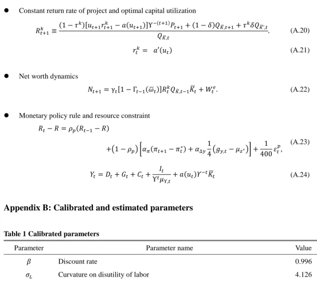
Constant return rate of project and optimal capital utilization 𝑅𝑅𝑡𝑡+1𝑘𝑘 ≡(1 − 𝜏𝜏 𝑘𝑘)[𝑢𝑢 𝑡𝑡+1𝑟𝑟𝑡𝑡+1𝑘𝑘 − 𝑎𝑎(𝑢𝑢𝑡𝑡+1)]Υ−(𝑡𝑡+1)𝑃𝑃𝑡𝑡+1+ (1 − 𝛿𝛿)𝑄𝑄𝐾𝐾�,𝑡𝑡+1+ 𝜏𝜏𝑘𝑘𝛿𝛿𝑄𝑄𝐾𝐾�’,𝑡𝑡 𝑄𝑄𝐾𝐾�,𝑡𝑡 . (A.20) 𝑟𝑟𝑡𝑡𝑘𝑘 = 𝑎𝑎′(𝑢𝑢𝑡𝑡) (A.21)
Net worth dynamics
𝑁𝑁𝑡𝑡+1= γ𝑡𝑡[1 − Γ𝑡𝑡−1(𝜔𝜔�𝑡𝑡)]𝑅𝑅𝑡𝑡𝑘𝑘𝑄𝑄𝐾𝐾�,𝑡𝑡−1𝐾𝐾�𝑡𝑡+ 𝑊𝑊𝑡𝑡𝑡𝑡. (A.22)
Monetary policy rule and resource constraint 𝑅𝑅𝑡𝑡− 𝑅𝑅 = 𝜌𝜌𝑝𝑝(𝑅𝑅𝑡𝑡−1− 𝑅𝑅) +�1 − 𝜌𝜌𝑝𝑝� �𝛼𝛼𝜋𝜋(𝜋𝜋𝑡𝑡+1− 𝜋𝜋𝑡𝑡∗) + 𝛼𝛼∆𝑦𝑦14 �𝑔𝑔𝑦𝑦,𝑡𝑡− 𝜇𝜇𝑧𝑧∗�� + 1 400 𝜀𝜀𝑡𝑡𝑝𝑝, (A.23) 𝑌𝑌𝑡𝑡= 𝐷𝐷𝑡𝑡+ 𝜇𝜇𝑡𝑡+ 𝐶𝐶𝑡𝑡+Υ𝑡𝑡𝐼𝐼𝜇𝜇𝑡𝑡 Υ,𝑡𝑡+ 𝑎𝑎(𝑢𝑢𝑡𝑡)𝛶𝛶 −𝑡𝑡𝐾𝐾� 𝑡𝑡 (A.24)
Appendix B: Calibrated and estimated parameters
Table 1 Calibrated parameters
Parameter Parameter name Value
𝛽𝛽 Discount rate 0.996
𝜎𝜎𝐿𝐿 Curvature on disutility of labor 4.126
𝛹𝛹𝐿𝐿 Disutility weight on labor 0.7705
𝜆𝜆𝑤𝑤 Steady-state markup, suppliers of labor 0.2
𝜇𝜇𝑧𝑧 Growth rate of the economy 0.41
𝛶𝛶 Trend rate of investment-specific technological change 0.42
𝛿𝛿 Depreciation rate on capital 0.015
𝛼𝛼 Power on capital in production function 0.40
𝜆𝜆𝑓𝑓 Steady-state markup, intermediate good firms 0.20
1 − 𝛾𝛾 Fraction of entrepreneurial net worth transferred to households 1-0.985
𝑊𝑊𝑡𝑡 Transfer received by entrepreneurs 0.005
𝜂𝜂𝑡𝑡 Steady-state government spending-GDP ratio 0.2
𝜋𝜋𝑡𝑡𝑡𝑡𝑡𝑡𝑡𝑡𝑡𝑡𝑡𝑡 Steady-state inflation rate (APR) 2.43
𝜏𝜏𝑐𝑐 Tax rate on consumption 0.08
𝜏𝜏𝑘𝑘 Tax rate on capital income 0.32
24
Table 2: Prior distribution
Prior distribution
Parameter name Parameter Prior dist Mean SD
Panel1. Economic parameters
Calvo wage stickiness 𝜉𝜉𝑤𝑤 Beta 0.375 0.100
Habit parameter 𝑏𝑏 Beta 0.700 0.150
Steady-state probability of default 𝐹𝐹(𝜔𝜔�) Beta 0.007 0.0037
Monitoring cost 𝜇𝜇 Bata 0.275 0.150
Curvature, utilization cost 𝜎𝜎𝑡𝑡 Beta 1.000 1.000
Curvature, investment adjust cost 𝑆𝑆′′ Gamma 4.000 1.500
Calvo price stickiness 𝜉𝜉𝑝𝑝 Beta 0.375 0.100
Policy weight on inflation 𝛼𝛼𝜋𝜋 Gamma 1.700 0.100
Policy smoothing parameter 𝜌𝜌𝑝𝑝 Beta 0.800 0.100
Price indexing weight on inflation target 𝜄𝜄 Beta 0.500 0.250
Wage indexing weight on inflation target 𝜄𝜄𝑤𝑤 Beta 0.500 0.250
Wage indexing weight on persistent technology growth 𝜄𝜄𝜇𝜇 Beta 0.500 0.250
Policy weight on output growth 𝛼𝛼∆𝑦𝑦 Gamma 0.125 0.050
Panel2. Shocks
Correlation among signals 𝜌𝜌𝜎𝜎,𝑛𝑛 Normal 0 0.5
Autocorrelation, price markup shock 𝜌𝜌𝜆𝜆𝑓𝑓 Beta 0.5 0.2
Autocorrelation, price of investment goods shock 𝜌𝜌𝜇𝜇𝜓𝜓 Beta 0.5 0.2
Autocorrelation, government 𝜌𝜌𝑡𝑡 Beta 0.5 0.2
Autocorrelation, persistent technology growth 𝜌𝜌𝜇𝜇𝑧𝑧 Beta 0.5 0.2
Autocorrelation, transitory technology 𝜌𝜌𝜖𝜖 Beta 0.5 0.2
Autocorrelation, risk shock 𝜌𝜌𝜎𝜎 Beta 0.5 0.2
Autocorrelation, consumption preference shock 𝜌𝜌𝜁𝜁𝑐𝑐 Beta 0.5 0.2
Autocorrelation, marginal efficiency of investment 𝜌𝜌𝜁𝜁𝐼𝐼 Beta 0.5 0.2
Autocorrelation, term structure shock 𝜌𝜌𝜂𝜂 Beta 0.5 0.2
Standard deviation, anticipated risk shock 𝜎𝜎𝜎𝜎,𝑛𝑛 Invg2 0.001 0.0012
Standard deviation, unanticipated risk shock 𝜎𝜎𝜎𝜎,0 Invg2 0.002 0.0033
SD. Measurement error on net worth 𝑆𝑆𝐷𝐷𝑚𝑚,𝑛𝑛 Weibull 0.01 5
Standard deviation, shock innovations
Price markup 𝜎𝜎𝜆𝜆𝑓𝑓 Invg2 0.002 0.0033
Investment price 𝜎𝜎𝜇𝜇𝜓𝜓 Invg2 0.002 0.0033
Government consumption 𝜎𝜎𝑡𝑡 Invg2 0.002 0.0033
Persistent technology growth 𝜎𝜎𝜇𝜇𝑧𝑧 Invg2 0.002 0.0033
Equity 𝜎𝜎𝛾𝛾 Invg2 0.002 0.0033
Temporary technology 𝜎𝜎𝜖𝜖 Invg2 0.002 0.0033
Monetary policy 𝜎𝜎𝜀𝜀𝑝𝑝 Invg2 0.583 0.825
Consumption preference 𝜎𝜎𝜁𝜁𝑐𝑐 Invg2 0.002 0.0033
Marginal efficiency of investment 𝜎𝜎𝜁𝜁𝐼𝐼 Invg2 0.002 0.0033
Term structure 𝜎𝜎𝜂𝜂 Invg2 0.002 0.0033
25
Table 3: Posterior distribution
Hirakata et al (2014) Hirose and Kurozumi (2012) Kaihatsu and Kurozumi (2014) Christiano et al (2014) This paper
Parameter Mean Mean Mean Mode Mode 90% confident interval
𝜉𝜉𝑤𝑤 - 0.567 0.497 0.81 0.7659 [0.7104,0.8185] 𝑏𝑏 0.8447 0.508 0.258 0.74 0.9009 [0.8619,0.9443] 𝐹𝐹(𝜔𝜔�) - - - 0.0056 0.0504 [0.0429,0.0583] 𝜇𝜇 0.0146 - - 0.21 0.1196 [0.1058,0.1341] 𝜎𝜎𝑡𝑡 - 4.411 0.475 2.54 1.0047 [0.1059.1.9117] 𝑆𝑆′′ 8.6739 7.118 0.425 10.78 10.4058 [8.6997,12.1906] 𝜉𝜉𝑝𝑝 0.6064 0.715 0.675 0.74 0.7688 [0.6994,0.8419] 𝛼𝛼𝜋𝜋 1.4832 1.694 1.652 2.40 1.6594 [1.5140,1.8130] 𝜌𝜌𝑝𝑝 - 0.794 0.749 0.85 0.8813 [0.8563,0.9055] 𝜄𝜄 0.0739 0.31 0.408 0.90 0.7321 [0.5342,0.9461] 𝜄𝜄𝑤𝑤 - 0.159 0.503 0.49 0.2854 [0.1934,0.3740] 𝜄𝜄𝜇𝜇 - - - 0.94 0.9800 [0.9576,0.9998] 𝛼𝛼∆𝑦𝑦 0.0238 0.0065 0.065 0.36 0.1264 [0.0427,0.2103] 𝜌𝜌𝜎𝜎,𝑛𝑛 - - - 0.39 0.4204 [0.2127,0.6415] 𝜌𝜌𝜆𝜆𝑓𝑓 0.68 0.933 0.976 0.91 0.9126 [0.8747,0.9459] 𝜌𝜌𝜇𝜇𝜓𝜓 - - 0.929 0.99 0.9956 [0.9926,0.9989] 𝜌𝜌𝑡𝑡 0.8045 0.945 0.991 0.94 0.8812 [0.7797,0.9807] 𝜌𝜌𝜇𝜇𝑧𝑧 - 0.0032 0.051 0.15 0.1564 [0.0427,0.2656] 𝜌𝜌𝜖𝜖 0.8719 - - 0.81 0.9681 [0.9536,0.9827] 𝜌𝜌𝜎𝜎 - - - 0.97 0.3244 [0.2124,0.4419] 𝜌𝜌𝜁𝜁𝑐𝑐 0.9145 0.91 0.858 0.90 0.1970 [0.0464,0.3361] 𝜌𝜌𝜁𝜁𝐼𝐼 0.377 0.461 0.999 0.91 0.9230 [0.8990,0.9474] 𝜌𝜌𝜂𝜂 - - - 0.97 0.9564 [0.9408,0.9725] 𝜎𝜎𝜎𝜎,𝑛𝑛 - - - 0.028 0.0181 [0.0138,0.0225] 𝜎𝜎𝜎𝜎,0 - - - 0.07 0.5084 [0.4122,0.6010] 𝑆𝑆𝐷𝐷𝑚𝑚,𝑛𝑛 - - - 0.018 0.0126 [0.0111,0.0140] 𝜎𝜎𝜆𝜆𝑓𝑓 0.0814 0.152 0.165 0.011 0.0060 [0.0040,0.0081] 𝜎𝜎𝜇𝜇𝜓𝜓 - - 0.4113 0.004 0.0014 [0.0012,0.0015] 𝜎𝜎𝑡𝑡 0.0256 0.454 0.517 0.023 0.0042 [0.0037,0.0048] 𝜎𝜎𝜇𝜇𝑧𝑧 - 1.632 1.291 0.0071 0.0031 [0.0027,0.0036] 𝜎𝜎𝛾𝛾 0.3736 - 1.39 0.0081 0.0002 [0.0002,0.0003] 𝜎𝜎𝜖𝜖 0.0111 - - 0.0046 0.0026 [0.0022,0.0029] 𝜎𝜎𝜀𝜀𝑝𝑝 0.0015 0.098 0.138 0.49 0.5829 [0.4625,0.6961] 𝜎𝜎𝜁𝜁𝑐𝑐 0.0019 4.996 - 0.023 0.0058 [0.0035,0.0082] 𝜎𝜎𝜁𝜁𝐼𝐼 0.0256 4.147 3.768 0.055 0.0147 [0.0105,0.0187] 𝜎𝜎𝜂𝜂 - - - 0.0016 0.0056 [0.0039,0.0070]
26
References
1. Adjemian, S., Bastani, H., Juillard, M., Mihoubi, F., Perendia, G., Ratto, M., Villemot, S., 2011.
Dynare: reference manual version 4. CEPREMAP, Dynare Working Papers 1.
2. Alexopoulos, M., 2011. Read All about It!! What Happens Following a Technology Shock? American
Economic Review, 101 (4): 1144–79.
3. Andolfatto, D., 1996. Business Cycles and Labor-Market Search. American Economic Review, 86 (1):
112–32.
4. An, S., Schorfheide, L, 2007. Bayesian Analysis of DSGE Models. Econometric Review, 26, 113-219.
5. Bayoumi, T., 2001. The morning after: explaining the slowdown in Japanese growth in the 1990s.
Journal of International Economics, 53 (2), 241–259.
6. Bernanke, B.S., Gertler, M., Gilchrist, S., 1999. The financial accelerator in a quantitative business
cycle framework. In: Taylor, J.B., Woodford, M. (Eds.), Handbook of Macroeconomics, vol. 1C. Elsevier, Amsterdam, pp. 1341–1393.
7. Blanchard, O.J., C.M., Kahn, 1980. The Solution of Linear Difference Models under Rational
Expectations. Econometrica, 48, 1305-1312.
8. Bloom, N., 2009. The Impact of Uncertainty Shocks. Econometrica, 77 (3): 623–85.
9. Calvo, G.A., 1983. Staggered prices in a utility-maximizing framework. Journal of Monetary
Economics, 12 (3), 383–398.
10. Christiano, L.J., Fujiwara, I., 2006. Bubbles, excess investments, working hour regulation, and lost decade. Bank of Japan Working Paper Series 06-J-8.
11. Christiano, L. J., Eichenbaum, M., Evans, C., 2005. Nominal Rigidities and the Dynamic Effects of a Shock to Monetary Policy. Journal of Political Economy, 113(1), 1-45.
12. Christiano, L. J., Ikeda, D., 2013. Leverage Restrictions in a Business Cycle Model. National Bureau of Economic Research Working Paper 18688.
13. Christiano, L.J., Motto, R., Rostagno, M.V., 2014. Risk shocks. American Economic Review, 104 (1), 27–65.
14. Davis, J. M., 2008. Noews and the Term Structure in General Equilibrium. In Three Essays in Macroeconomics, 9-57, PhD diss., Northwestern University.
15. De Graeve, F., 2008. The External Finance Premium and the Macroeconomy: US Post-WWII Evidence, Journal of Economic Dynamics and Control, 32, 3415-3440.
27
16. Eberly, J., Sergio R., 2012. What explains the lagged-investment effect? Journal of Monetary Economics, 59, 370-380.
17. Erceg, C. J., Henderson, D. W., Levin, A. T., 2000. Optimal Monetary Policy with Staggered Wage and Price Contracts. Journal of Monetary Economics, 46 (2), 281-313.
18. Fujiwara, I., Hirose, Y., Shintani, M., 2008. Can News Be a Major Source of Aggregate Fluctuations? A Bayesian DSGE Approach. IMES Discussion Paper Series 08-E-16, Institute for Monetary and Economic Studies, Bank of Japan.
19. Gertler, M., Karadi, P., 2011. A Model of Unconventional Monetary Policy. Journal of Monetary Economics, 58, 17-34.
20. Gertler, M., Kiyotaki, N., 2011. Financial Intermediaries and Monetary Economics. Handbook of Monetary Economics, ed. Benjamin Friedman and Michael Woodford. Amsterdam, New York and Oxford: Elsevier Science, North-Holland.
21. Hayashi, F., Prescott, E.C., 2002. The 1990s in Japan: the lost decade. Review of Economic Dynamics, 5 (1), 206–235.
22. Hirakata, N., Sudo, N., Ueda, K., 2011. Do banking shocks matter for the U.S. economy? Journal of Economic Dynamics, Control 35 (12), 2042–2063.
23. Hirose, Y., Kurozumi, T., 2012. Do investment-specific technological changes matter for business fluctuations? evidence from Japan. Pacific Economic Review, 17 (2), 208–230.
24. Justiniano, A., Primiceri, G.E., Tambalotti, A., 2011. Investment shocks and the relative price of investment. Review of Economic Dynamics, 14 (1), 102–121.
25. Kaihatsu, S., Kurozumi, T., 2014. What caused Japan’s Great Stagnation in the 1990s? Evidence from an estimated DSGE model. Journal of the Japanese and International Economies, Elsevier, 34(C), 217-235.
26. Kawamoto, T., 2004. What Do the Purified Solow Residuals Tell Us about Japan’s Lost Decade? IMES Discussion Paper Series, No. 2004-E-5.
27. Levin, A., Onatski, A., Williams, J., Williams, N., 2005. Monetary Policy under Uncertainty in Micro-Founded Macroeconometric Models. In: NBER Macroeconomics Annual, 20, 229-287.
28. Lucca, D. O., 2006. Essays in Investment and Macroeconomics. Phd dissertation, Northwestern University, Department of Economics.
28
29. Matsuyama, K., 1984. A Learning Effect Model of Investment: An Alternative Interpretation of
Tobin’s Q. unpublished manuscript, Northwestern University, available at
http://faculty.wcas.northwestern.edu/~kmatsu/ALearningEffectModel.pdf
30. Merz, M., 1995. Search in the Labor Market and the Real Business Cycle. Journal of Monetary Economics, 36, 269-300.
31. Motonishi, T., Yoshikawa, H., 1991. Causes of the Long Stagnation of Japan during the 1990s: Financial or Real? Journal of the Japanese and International Economies, 13, 181-200.
32. Ogama, K., 2007. Debt, R&D investment and technological progress: a panel study of Japanese manufacturing firms’ behavior during the 1990s. Journal of the Japanese and International Economies, 21(4), 403-423.
33. Ramey, V.A., 2011. Identifying Government Spending Shocks: It’s All in the Timing. Quarterly Journal of Economics, 126 (1): 1–50.
34. Sims, C.A., 2002. Solving Linear Rational Expectation Models. Computational Economics, 20, 1-20. 35. Smets, F., Wouters, R., 2003. An Estimated Dynamic Stochastic General Equilibrium Model of the
Euro Area. Journal of the European Economic Association, 1(5), 1123-1175, 09.
36. Smets, F., Wouters, R., 2007. Shocks and frictions in US business cycles: a Bayesian DSGE approach. American Economic Review, 97 (3), 586–606.
37. Sugo, T., Ueda, K., 2008. Estimating a dynamic stochastic general equilibrium model for Japan. Journal of the Japanese and International Economy, 22 (4), 476–502.
38. Topel, R., Rosen, S., 1988. Housing Investment in the United States. Journal of Political Economy, 96 (4), 718-740.
39. Watanabe, W., 2007. Prudential Regulation and the “Credit Crunch”: Evidence from Japan. Journal of Money, Credit and Banking. 39(2-3), 639-665.
29
Figure 1: The transition of GDP of Japan
Note: GDP is an actual GDP growth rate (seasonally adjusted) from the Cabinet Office of Japan. Shaded areas are recession periods, according to the Reference Dates of Business Cycle, the Cabinet Office of Japan.
time 1980 1985 1990 1995 2000 2005 2010 Percentage point -10 -5 0 5 10 GDP(annual rate) Recession
30 1990 1995 2000 2005 2010 Percent -5 -4 -3 -2 -1 0 1 2 3 4 5 A. GDP
Actual data (left side) Historical decomposition by technological shock alone (right side)
1990 1995 2000 2005 2010 Percent -3 -2 -1 0 1 2 3 4 B. Consumption 1990 1995 2000 2005 2010 Percent -10 -5 0 5 10 C. Investment -1 0 1 2 3 4 5 6
Figure 2: The comparison between time series of the selected data and those of corresponding endogenous variables calculated by the estimated TFP shock
1990 1995 2000 2005 2010 Percent -5 -4 -3 -2 -1 0 1 2 3 4 5 A. GDP
Actual data (left side)
Histrical decomposition by M.E.I. shock alone (right side)
1990 1995 2000 2005 2010 Percent -5 -4 -3 -2 -1 0 1 2 3 4 5 B. Consumption 1990 1995 2000 2005 2010 Percent -10 -8 -6 -4 -2 0 2 4 6 8 10 C. Investment -20 -15 -10 -5 0 5 10 15 20
Figure 3: The comparison between time series of the selected data and those of corresponding endogenous variables calculated by the estimated Marginal Efficiency of Investment shock
31
Figure 4: The comparison between time series of the selected data and those of corresponding endogenous variables calculated by the estimated risk shock
1990 1995 2000 2005 2010 Percent -5 -4 -3 -2 -1 0 1 2 3 4 5 A. GDP
Historical decomposition by risk shock alone (right side) Actual data (left side)
1990 1995 2000 2005 2010 Percent -5 -4 -3 -2 -1 0 1 2 3 4 5 B. Consumption 1990 1995 2000 2005 2010 Percent -10 -8 -6 -4 -2 0 2 4 6 8 10 C. Investment -1 -0.8 -0.6 -0.4 -0.2 0 0.2 0.4 0.6 0.8 1
32
Figure 5: Time path of the estimated risk shock
Note: Shaded areas are recession periods, according to the Reference Dates of Business Cycle, the Cabinet Office of Japan.
Table 4: Correlation coefficient with model out-of-sample indicators
Correlation coefficient
Coefficient of variation of Nikkei 225 0.22184
SD of DI for business condition
All industries -0.34288
Manufacture -0.26073
Non-Manufacture -0.39565
DI for business condition -0.72149
DI for business condition (prediction) -0.71395
DI for financial position -0.69687
DI for lending attitude -0.63490
a quatery
1990 1995 2000 2005 2010
deviation from the steady state value (% point)
-2 -1.5 -1 -0.5 0 0.5 1 1.5 2 2.5 3
risk variation in the model a period of recession