9. Retrospective Voting at the Macro Level
権利
Copyrights 日本貿易振興機構(ジェトロ)アジア
経済研究所 / Institute of Developing
Economies, Japan External Trade Organization
(IDE-JETRO) http://www.ide.go.jp
シリーズタイトル(英
)
Occasional Papers Series
シリーズ番号
41
journal or
publication title
Electoral Volatility in Turkey - Cleavages vs.
the Economy
page range
105-130
year
2007
9
Retrospective Voting at
the Macro Level
While the Turkish party system has recently become solidly anchored to major social cleavages, as shown in Chapter 6 and Chapter 7, total electoral volatility has not declined correspondingly. This is because the electoral volatility stemming from retrospective voting has increased, particularly since the 1990s (Figure 3-1 and Figure 3-2). The retrospective voting model in general assumes that the electorate evaluates the incumbent based on economic performance in the recent past, as shown by Section 1.3 of Chapter 1. Does this model apply to Turkey?
This chapter investigates the relationship between changes in macroeconomic vari-ables (real per capita GNP, unemployment, and inflation) and changes in support for the incumbent party/parties. The first part of the chapter discusses the choice and compilation of dependent and independent variables. Second, a time-series analysis is performed on the retrospective voting model thus derived. The third part tests indi-vidual elections using the cross-sectional model of retrospective voting, with the province as the unit of analysis.
9.1. The Choice of the Dependent Variable: Support or Swing?
The retrospective voting model posits that people make voting decisions based on the past performance of the incumbent. The model, whether time-series or cross-sec-tional, measures the relationship between the governing party’s/parties’ vote percent-age in the election concerned and economic indicators or voters’ perceptions of economic conditions in the period of twelve months or less immediately preceding the election. This study adopts as the dependent variable changes in the party’s/ parties’ vote percentage between two consecutive elections, hereafter called “vote swing,” which constitutes the dominant portion of electoral volatility.
There are both conceptual and methodological reasons for using change rather than level as the dependent variable for this study. Conceptually, the major concern of this study is voters’ reactions to government performance, or the cost of ruling (the incumbent vote swing) (Palmer and Whitten 2002, p. 73), rather than the level of incumbent support. Methodologically, the clear declining trend in incumbent votes required data transformation through differentiation. The following paragraphs ex-plain the reasons for and the processes of data transformation.
When dealing with time-series data for a linear regression, it is necessary, first, to ascertain whether the dependent variable is influenced by time. Linear regressions assume constant mean and variance for the error term, which is the difference be-tween the real and the predicted value of the dependent variable. Time-series data often violate this “stationarity” assumption, due to their very nature, i.e., that the value at the current time point often strongly depends on the value at the previous time point.
The unit-root test shows whether the mean and variance of the data vary signifi-cantly across time. If they do, the data are called nonstationary. Nonstationary data are strongly autocorrelated with the first lag. The vote data used by Çarko%glu (1997), which represent the level of support for the incumbent party/parties in various elec-tions1 have a clear declining trend and are thus nonstationary (Figure 9-1). The Augmented Dickey-Fuller (ADF) unit-root test, when applied to this time-series data, fails to reject the null hypothesis that the time series is nonstationary (p= 0.272). The vote data thus violates the stationarity assumption for the time-series dependent variable.
Conventionally, nonstationary data can be transformed into stationary data through differentiation. For this study, however, it is more appropriate to use the vote swing for the incumbent party/parties between two consecutive elections (Figure 9-2) rather
0 10 20 30 40 50 60 70 1950 ’54 ’63 ’65 ’68 ’73 ’77 ’84 ’87 ’91 ’95 (%)
Fig. 9-1. Votes for the Incumbent Party/Parties, 1950–95
than the difference between incumbent votet and incumbent votet-1 since incumbents may change between two elections (at time t and time t− 1). The results of the ADF test suggest2 that the new time series thus created is stationary (p= 0.01, maximum lag= 5), with the mean and variance constant and independent of time.3
After stationarity is confirmed, the second step is to check for autocorrelation by correlogram. Whereas the unit-root test ensures that the autocorrelation of the time-series data is not too high (i.e., lower than one), the correlogram analysis measures the degree of autocorrelation. The correlogram of the vote swing data reveals no statisti-cally significant autocorrelation for any of the lags. It is consequently justifiable to use the vote swing data as the dependent variable. The time-series multiple regression, when applied to the data set for which the vote data are replaced with the vote swing data, shows that none of the independent variables (percent change in per capita GNP, unemployment rate, or inflation rate) are related to changes in electoral support for the incumbent party/parties.
9.2. Per Capita Economic Growth Rate: Fluctuations
As the dependent variable requires careful scrutiny, so do the independent variables, which in this study are represented by economic indicators. Regression analysis in theory postulates no assumptions on the distribution of independent variables. In practice, however, trends and fluctuations in time-series independent variables can blur their relationships with the dependent variable.4 It is also necessary at the outset to ensure that economic data are measured validly and reliably over time.5 An exami-nation of time-series data for real per capita economic growth, inflation, and
unem-−50 −40 −30 −20 −10 0 10 1950 ’57 ’65 ’69 ’77 ’87 ’91 ’95 2002
Fig. 9-2. Vote Swing for the Incumbent Party/Parties, 1950–2002
Source: Compiled by the author from Appendix VI.
Notes: 1. Vote swing is represented by change in the incumbent vote percentage. 2. The number of observations is smaller than in Çarko%glu’s article (1997)
since they excluded senate elections and by-elections (both parliamen-tary and local) although they included the more recent 1999 and 2002 general elections.
ployment reveals that these variables cannot be used for analysis without modifica-tion.
First, for Turkey, the last-year value of economic growth cannot always be a valid measurement of voter grievances. The reason lies in the country’s highly erratic economic growth,6 compared with the major Western democracies (Figure 9-3 and Figure 9-4). Until the 1960s, Turkey’s dominantly agricultural economy was very unstable due to its susceptibility to changes in weather conditions. The transition beginning in the 1960s to a planned economy geared to import-substitution industrial-ization somewhat reduced the instability. Fluctuations in economic growth, however, increased again beginning in the late 1980s, when it substantially liberalized its capital account.7 The government encouraged the inflow of (short-term) foreign capi-tal by keeping the Turkish lira overvalued8 while at the same increasing its depen-dence on the capital market to finance its fiscal deficits. The overvaluation of the lira, however, often led to a larger current account deficit, which was only sustainable until forced devaluations in the form of currency crises such as in 1994 and 2001. These crises9 radically reduced the economic growth rates.
In politics, a sudden jump in economic growth in an election year does not signifi-cantly calm voter resentment that has accumulated during the previous years of stagnant or negative economic growth.10 In the Western democracies, the real per capita economic growth rate already reflected, to a significant extent, its previous value. The degree of association between the current year’s value and the previous value can be measured by autocorrelation coefficients. The correlograms of real economic growth data for the Western democracies in Table 9-1 reveal that for almost
−10 −5 0 5 10 15 1961 ’65 ’69 ’73 ’77 ’81 ’85 ’89 ’93 ’97 ’01
France Germany Italy UK USA Turkey
Fig. 9-3. Real Per Capita Economic Growth Rate: Western Democracies and Turkey, 1961–2002
Source: Compiled by the author from IMF (2003).
Note: In accordance with the availability of comparable data, economic growth is mea-sured by GDP.
all the countries, the series are positively autocorrelated with (at least) the first lag, which represents the value for the previous year. But for Turkey, the autocorrelation coefficient is negative, though not statistically significantly so.
In such a situation, the current year’s value of economic data should be imbued with previous values. High economic growth in an election year may be a reaction to low economic growth in the previous year, and low economic growth may occur due to the saturation of a period of high economic growth. In this study, the real per capita GNP growth rate for a given year was added to the corresponding value for the previous year and the sum was divided by two. This process in essence controlled for the rate of economic growth that preceded the election year. Only the first lag (the
0 0.5 1 1.5 2 2.5 3 3.5 4 4.5 5
France Germany Italy UK U.S.A. Turkey (%)
Fig. 9-4. Standard Deviation of the Real Per Capita Economic Growth Rate: Western Democracies and Turkey, 1961–2002
Source: See Figure 9-3.
Note: In accordance with the availability of comparable data, eco-nomic growth is measured by GDP.
TABLE 9-1
FIRST-ORDER AUTOCORRELATIONOFTHE REAL PER CAPITA ECONOMIC GROWTH RATE:
WESTERN DEMOCRACIESAND TURKEY, 1961–2002
Country Autocorrelation Q-Stat. Prob. France |***** 0.592 15.817 0.000 Germany |** 0.246 2.7184 0.099 Italy |** 0.285 3.6713 0.055 United Kingdom |** 0.267 3.2218 0.073 United States |** 0.198 1.7629 0.184 Turkey *| −0.163 1.1642 0.281 Source: Calculated and compiled by the author from IMF (2003).
Note: Includes Turkey and major Western democracies (Germany, the United States, France, United Kingdom, and Italy), for each of which retrospective voting was confirmed in Norpoth, Lewis-Beck, and Lafay (1991).
value for one year earlier) was used, considering that for most of the Western democ-racies, there is only a first-order autocorrelation for the real GNP growth rate, as shown above.
9.3. Unemployment: Trends, Extrapolation, and Definition
The unemployment data for Turkey requires caution for two main reasons. First, there is a long-term upward trend that stems from Turkey’s industrialization and urbaniza-tion processes (Figure 9-5). The unemployment rate, as defined in Turkey, is lower in rural areas than in urban areas, because unpaid family workers, which are by definition included in employment statistics, form the largest portion of the employed in rural areas (Figure 9-6). Since the majority of the unpaid family workers are employed in agriculture, the decline of that sector reduced this type of employment and thus increased unemployment.11 In Western democracies, unemployment also exhibited an upward trend during the corresponding period.
Methodologically, for both Turkey and Western democracies, these long-term trends in independent variables may distort the real relationship even if the dependent variable has no trend.12 It is more appropriate to use change in, rather than the level of, unemployment.13 Then, what time span should be applied to changes in the unem-ployment rate as an independent variable for the Turkish model? For both Turkey and the Western democracies, changes in the unemployment rate are positively auto-correlated with their first lag (Table 9-2). This fact justifies the use of changes in the unemployment rate for the last year in the Turkish case as well, since the last year’s value reflects that of the previous year. Thus, unlike economic growth data, for
0 2 4 6 8 10 12 1945 ’50 ’55 ’60 ’65 ’70 ’75 ’80 ’85 ’90 ’95 2000 (%)
Fig. 9-5. Unemployment Rate in Turkey, 1945–2002
Sources: Bulutay (1995, p. 256, table 8.A); SIS, Labour Statistics, various years. Note: Percentage unemployed to the total civilian labor force.
unemployment data it is not necessary to use the mean for the last two years. While it is desirable to use changes in the unemployment rate, change-based data requires more precision than level-based data. In fact, it is doubtful whether unem-ployment data in Turkey before 1988 are sufficiently accurate. The State Institute of Statistics (SIS) has conducted systematic labor force surveys since 1988. However, before then, samples for labor force statistics were limited and thus failed to represent Turkey as a whole. The only long-term data available for the pre-1988 period was compiled by Bulutay (1995), who extrapolated unemployment rates for the 1923– 1988 period from per capita investment, using the 1988 Labor Force Survey as a structural basis.14 As shown by the data, yearly changes in unemployment were mostly less than 1 percent, while levels of unemployment ranged from 3 to 10 percent.
0 5 10 15 20 25 30 35 1991 ’92 ’93 ’94 ’95 ’96 ’97 ’98 ’99 2000 ’01 ’02 (%)
Fig. 9-6. Unpaid Family Workers to Total Employment, 1991–2002
Source: SIS, Household Labour Force Survey Results, various years. TABLE 9-2
FIRST-ORDER AUTOCORRELATIONFOR UNEMPLOYMENT RATE CHANGE: WESTERN DEMOCRACIESAND TURKEY, 1986–2002
Country Autocorrelation Q-Stat. Prob. France |****** 0.724 10.059 0.002 Germany |******* 0.870 14.529 0.000 Italy |****** 0.774 11.508 0.001 United Kingdom |***** 0.628 7.5618 0.006 United States |****** 0.748 10.737 0.001 Turkey |**** 0.475 4.3337 0.037 Source: Calculated and compiled by the author from Organisation for Economic Co-operation and Development, Main Economic Indicators (Paris: OECD, various years).
Note: The ADF test showed that all the time series were stationary. Second- and lower-order partial autocorrelation coefficients for these countries are negative, weak, or insignificant.
An error margin of 1 percentage point in the unemployment data thus can easily change the fluctuation in the unemployment rate from positive to negative. One cannot expect this data to have sufficient precision to distinguish changes in unem-ployment from one year to the next.15
Second, employment statistics for Turkey since 1989 contain “underemployment” figures ranging approximately from 6 to 8 percent (Figure 9-7). The underemployed are defined by the SIS as either “persons who work less than 40 hours because of economic reasons during the reference period and are able to work more at their present job or are capable of doing a further job” or “persons who are not in the above group want to change his/her present job or are seeking a further job because of an insufficient income or because of not working in his/her usual occupation.”16 Thus, the substantial number of underemployed persons as well as unpaid family workers in the unemployed category makes the definition of unemployment much narrower than those in the Western democracies. Moreover, the rates of underemployment and unemployment do not necessarily change in the same direction, though they do not always move in the opposite direction, either. In fact, neither pattern holds. The results of a regression analysis with semi-annual data for the 1989–2002 period show that changes in the unemployment rate were not related to the underemployment rate at a statistically significant level.17 Combining the unemployment and underemployment rates therefore does not solve the problem.
In the following analysis, the first problem is mitigated by treating the pre-1988 and post-1988 periods separately. The second problem needs to be dealt with only if the more reliable post-1988 unemployment data are found not to show the expected effect on change in incumbent votes.
Fig. 9-7. Unemployment and Underemployment, 1988–2002 Semiannual
Sources: SIS, Household Labour Force Survey Results, various years. Note: Underemployment data is available from 1989.
0 2 4 6 8 10 12 1988 ’91 ’94 ’97 2000 Unemployment Underemployment (%)
9.4. Inflation: Indexation and Inertia
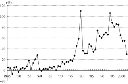
As with the unemployment rate, the inflation rate has a strong upward trend (Figure 9-8). For the same reason, therefore, it is appropriate to use change in the inflation rate. The ADF test, when applied to this time-series data, fails to reject the null hypothesis that the time series is nonstationary (p= 0.222). The same test shows that the first difference of the time series, i.e., change in the inflation rate (Figure 9-9), is stationary (p= 0.0001).
Changes in inflation reflect the erosion of real income more accurately than its level when inflation is continuously high and thus inertial. Turkish inflation became inertial in the 1980s (Sakallıo%glu and Yeldan 1999; Erlat 2001). It subsequently became a fact of life and was generally accepted as long as it did not accelerate substantially. Behind this inertia were indexation mechanisms, such as that for rent, which mitigated the impacts of price increases in the past (Central Bank of the Republic of Turkey [2000]).18 Although the indexation mechanism partially alleviated the social costs of inflation, it also allowed the inflationary momentum to continue. Thus, the prevalence of inertial inflation justified the use of a change-based variable instead of a level-based variable for inflation.
A question still remains, however, regarding the time span of the variable. As was already shown above, the values of certain economic indicators reflect their previous value. These autocorrelated, although stationary, data have been used for
retrospec-−20 0 20 40 60 80 100 120 1945 ’50 ’55 ’60 ’65 ’70 ’75 ’80 ’85 ’90 ’95 2000 (%)
Fig. 9-8. Inflation in Turkey, 1945–2002
Source: Compiled by the author from IMF (2003).
Note: Inflation was measured by percentage change in the consumer price in-dex.
tive voting analyses of industrial democracies.19 The results of the correlograms show that for the Western democracies, inflation rates were invariably positively autocorrelated with their first lag (Table 9-3). For Turkey, on the other hand, changes in the inflation rate were negatively autocorrelated at the 0.10 significance level (r= 0.239, p = 0.088). It is desirable therefore to use the mean for the last two years for changes in the inflation rate, in the same way as for the real per capita GNP growth rate, so that the value for the last year of the incumbency reflects the value for the previous year. −80 −60 −40 −20 0 20 40 60 1946 ’51 ’5 6 ’61 ’66 ’71 ’76 ’81 ’86 ’91 ’96 2001
Fig. 9-9. Change in the Inflation Percentage, 1946–2002
Source: Compiled by the author from IMF (2003).
Note: Inflation was measured by percentage change in the consumer price index. TABLE 9-3
FIRST-ORDER AUTOCORRELATIONOF INFLATION RATES: WESTERN DEMOCRACIESAND TURKEY, 1949–2002
Country Autocorrelation Q-Stat. Prob. France |***** 0.599 20.141 0.000 Germany |** 0.296 4.9257 0.026 Italy |****** 0.787 35.330 0.000 United Kingdom |****** 0.781 34.762 0.000 United States |***** 0.705 28.386 0.000 Turkeya **| −0.239 2.9164 0.088
Source: Calculated and compiled by the author from IMF (2003).
Note: The ADF test showed that all the time series were stationary. Second- and lower-order partial autocorrelation coefficients for these countries are generally weak or insignificant.
9.5. A Time-Series Analysis with Modified Data
This section provides the results of a time-series regression testing the effects of (1) the real per capita GNP growth rate for the last two years before the election, (2) change in the unemployment rate for the election year, and (3) change in the inflation rate for the last two years before the election, on changes in the governing party/ parties’ vote percentage between two consecutive elections. The compilation process of these three independent variables was extensively discussed in the previous section and is summarized in Table 9-4. When the election took place in the first six months of the year, the previous year’s value is used as the value for the election year and the value for the year before that is used as the value for the year before the election.
The dependent variable is change in incumbent vote percentage, with the incum-bent being defined as the last incumincum-bent party/parties that ruled for at least a year before the general election was held. Previous studies showed that the type of incum-bent governments (ranging from single-party to minority) as well as the weight of the political responsibility of coalition parties within the cabinet affected the extent of punishment of by the voters (Powell and Whitten 1993). However, given the small sample, it is difficult to take all these variables into consideration since it engenders the problem of “too many variables for too few cases.” The votes for the coalition parties are thus summed up for the calculation of incumbent votes. Since this sum-ming approach produced the expected results, a more differentiated approach was not taken.
Two control variables are included among the independent variables. One is the
TABLE 9-4
SUMMARYOFTHE ECONOMIC DATA SERIES, 1945–2002
Standard First-Order Time-Series Variable Mean Deviation Autocorrelation (r) Compilation Change in real per 2.317 4.361 Not significant Last-two-year
capita GNP mean
Change in 0.635 17.284 Negative Last-two-year the inflation ratea (−0.239*) mean
Change in the 0.139 0.662 Positive Last-year unemployment rate (0.291**) value
Source: Compiled by the author from the sources cited in Appendix VI.
Notes: 1. This table summarizes the (stationary) time-series economic data, from which the inde-pendent variables were derived, in terms of (1) descriptive statistics, (2) autocorrelation patterns, and (3) the method of time-series compilation. When the series was not posi-tively autocorrelated with any of its lags, such as for real per capita GNP growth or change in the inflation rate, the mean value for the last two years before the election was used. When the series was positively autocorrelated with its first lag, such as for change in the unemployment rate, then the last-year value was used.
2. All variables are shown in percentage.
a The inflation rate was measured by percentage change in the consumer price index. *p< 0.10, **p< 0.05.
number of years between the inauguration of the government and the following general election. The other is the number of political parties in the government. First, the vote swing for the incumbent party/parties is negatively affected by the number of years in incumbency due to the effect of the “cost of ruling.” The longer the period in power, the greater the loss of votes for the incumbent party/parties. Second, it takes more votes to form a coalition government than a single-party government. This is because the first party obtains more seats per vote than the other smaller parties, even under proportional representation. If a government includes any parties smaller than the first party, then the total number of votes required to form a government should be larger than the total number of votes required for a single-party government. Change in incumbent votes between two elections thus is expected to be larger for a coalition government than for a single-party one.
The sample space (N= 17) consists only of general elections of the national assem-bly and of the provincial assemblies from 1950 to 2002. By-elections of the national assembly, the senate (until 1980)20 and local by-elections, which were included in Çarko%glu (1997), are excluded from the current study since these elections did not take place in all the provinces and thus did not accurately represent electoral support across time and space.
The results of a multiple regression with modified economic variables (Table 9-5) show that the percentage change in real per capita GNP accounted for changes in incumbent vote percentage at a statistically significant level. The two other economic variables had statistically insignificant regression coefficients, while the two control
TABLE 9-5
RETROSPECTIVE VOTING MODELFOR TURKEY, 1950–2002 (N= 17)
Independent Variable Coefficient Std. Error t-Statistic Prob. VIFa
Intercept −0.144 6.226 −0.023 0.982
Change in real per capita GNP, 2.478 0.622 3.983 0.002 1.175 last-two year mean (%)
Change in unemployment rate, 1.668 2.634 0.633 0.540 1.175 last year (%)
Change in inflation rate, 0.052 0.192 0.271 0.791 1.264 last-two year mean (%)
Number of years in office −3.346 1.556 −2.151 0.055 1.120 Number of governing parties −4.591 2.335 −1.967 0.075 1.160
R2 0.700 Mean dependent var. −7.471
Adjusted R2 0.564 S. D. dependent var. 10.50
S. E. of regression 6.934 Akaike info. criterion 6.981 Sum squared resid. 528.9 Schwarz criterion 7.275 Log likelihood −53.34 F-statistic 5.144 Durbin-Watson stat. 2.536 Prob. (F-statistic) 0.011 Source: Compiled by the author from Appendix VI.
Notes: The dependent variable is the vote swing for the incumbent party/parties between two con-secutive elections.
a Multicollinearity is suspected if variance inflation factor (VIF) exceeds 10. ** p< 0.05, *** p< 0.01.
variables had the expected effects. This unsatisfactory performance of the regression model did not result from the temporal compilation of economic variables. When multiple regressions were run with the last-year value for all three economic vari-ables, which is the conventional approach to retrospective voting, none of their regres-sion coefficients were statistically significant.
9.6. Why GNP but Not Inflation or Unemployment?
Although the above model shows that real per capita GNP change was a strong predictor of the vote swing, why do unemployment and inflation fail to explain it? At this stage, two speculations can be made. First, with regard to unemployment, it may have been inappropriate to generate a change variable from extrapolated data for the pre-1988 period. As was explained in the above Section 9.3, the extrapolation method used by Bulutay (1995) was theoretically adequate for generating the yearly level of unemployment using census data at five-year intervals. Extrapolating change in em-ployment, however, is much more difficult. The margin of error is greater for changes in unemployment than for the unemployment level, which has a trend and thus is strongly determined by the previous value. The contamination effect of the extrapola-tion correlates is also greater for change in unemployment than for the unemployment level.
In fact, the unemployment data until 1987 and the vote swing display a pattern that is contrary to the theoretical expectation. A rise in the unemployment rate increased incumbent votes (Figure 9-10). This consistent relationship indicates that the pre-1988 unemployment data was systemically affected by the extrapolation process. Indeed, a further examination reveals that changes in the unemployment rate during the pre-1988 period were positively correlated with the real per capita GNP growth rate (Figure 9-11) while in theory, economic growth reduces unemployment. From the outset, the lack of collinearity between economic growth and changes in unem-ployment in the retrospective voting equation for Turkey is rather strange. The truth of the matter is that there was a negative relationship between the two variables for the post-1988 period but that the relationship was cancelled out by the seemingly positive relationship for the pre-1988 period. The spurious relationship for the pre-1988 pe-riod is due to the negative relationship between changes in the population growth rate and in the unemployment rate (Table 9-6).
On the other hand, the relation between the post-1988 unemployment data, which were actually measured rather than extrapolated, and the incumbent vote swing indi-cates that a rise in unemployment did increase the loss of incumbent votes (Figure 9-12). This shows that unemployment, in reality, was a critical determinant of retrospec-tive voting. Changes in the unemployment rate for the post-1988 period were also negatively related to changes in real per capita GNP (Figure 9-13), which accords with the economic theory that economic recessions increase unemployment.
Second, for inflation, a tentative speculation can be made. Under high and/or inertial inflation, what matters to wage earners and pensioners are inflation
adjust-−10 −5 0 5 10 15 20 −1.0 −0.5 0.0 0.5 1.0 1.5 2.0 2.5
Change in percentage unemployed
Residual change in the incumbent vote percentage
Fig. 9-10. Spurious Relationship between Change in the Extrapolated Unemployment Rate and the Residual Vote Swing, 1950–87 (N= 11)
Source: Compiled by the author from Appendix VI.
Note: The effect of the control variables (the number of incumbent parties and the number of years in incumbency) was subtracted from changes in the incumbent vote percentage.
ments for their fixed incomes rather than the level of or change in inflation per se. The preceding results suggest that inflation adjustments did not accurately reflect inflation on a yearly basis. The extent of inflation adjustments can be measured by changes in real wages, and there are indications that changes in real wages induced retrospective voting. In other words, a larger decline in real wages led to a larger loss of votes for the incumbents. Table 9-7 shows the results of the bivariate regression with White’s heteroscedasticity-consistent standard errors and covariance,21 showing that change in real wages was positively (though weakly) related to the vote swing residual (r= 0.149, p= 0.084). Change in real wages for each year was used since the time series was positively autocorrelated with its first lag (r= 0.366, p = 0.007) for the 1950– 2002 period, thus reflecting the previous year’s value.
Indeed, change in inflation was not a very decisive factor for change in real wages (Table 9-8).22 Change in real wages was primarily related to its first lag. Although change in real wages was secondarily (negatively) affected by change in inflation, there were other forces that determined them (Figure 9-14). Until 1980, yearly gains and losses in real wages occurred cyclically and relatively unintentionally. Since 1980, however, changes in real wages have been heavily influenced by government policy. From 1980 to 1986, real wages were severely restrained due to the IMF-supported stabilization program that sought to increase exports by lowering labor costs and the foreign exchange rate. Under the military government (1980–83), trade union activities were prohibited. The transition to a fully competitive election in 1987
alarmed the governing ANAP, which since 1983 had been responsible for economic austerity, and it adopted a more generous wage policy and raised real wages. Distinct rises in real wages coincided with general elections in 1987 and 1991 and the general local election in 1989. While the temporary decline in 1992 was a reaction to the previous large increases, consistent negative residuals since the mid-1990s were due to the IMF-prescribed structural adjustment policy that was intermittently imple-mented beginning from the economic crisis in 1994.23 These results imply that not even change in inflation, to say nothing of inflation per se, accurately reflected the level of grievances among wage earners.24
In sum, the foregoing analysis demonstrated that changes in real per capita GNP 0 1 2 3 4 5 6 7 8 9 −1.0 −0.5 0.0 0.5 1.0 1.5 2.0 2.5
Change in percentage unemployed
Percentage change in real GNP per capita
Fig. 9-11. Change in Real Per Capita GNP and Change in the Extrapolated Unemployment Rate, 1950–87 (N= 11)
Source: Compiled by the author from Appendix VI. TABLE 9-6
POPULATION GROWTHAND CHANGEINTHE UNEMPLOYMENT RATE, 1970–87
Independent Variable Coefficient Std. Error t-Statistic Prob. Population growth (%) −2.298 0.722 −3.184 0.005
R2 0.350 Mean dependent var. 0.128
Adjusted R2 0.351 S.D. dependent var. 0.690
S.E. of regression 0.556 Akaike info criterion 1.718 Sum squared resid. 5.256 Schwarz criterion 1.767 Log likelihood −14.461 Durbin-Watson stat 1.491
Source: Compiled by the author from IMF (2003).
Note: The dependent variable is change in the unemployment rate. The data is annual.
and in unemployment affected the vote swing. Changes in inflation did not display the expected effect.
9.7. Before and after 1980: Economic Growth and Retrospective Voting
These results provide evidence that punishment of the incumbent, i.e., vote swings from the incumbent to opposition parties, was indeed influenced by the government’s handling of the economy, with the economic growth rate being the most reliable predictor. It can be recalled, in the meantime, that while cleavage-type volatilities declined from the pre- to the post-1980 period, retrospective-type volatilities in-creased between these periods. Is it then possible to explain the growing extent of retrospective voting in post-1980 Turkey by the deterioration of the economy in the same period? Although rigorous statistical testing is not feasible due to the limited time points in the data, this section makes a preliminary comparison between the pre-and post-1980 periods in terms of economic growth pre-and retrospective-type volatili-ties.
There are limitations to any attempt to establish any relationship between the decline in economic growth and the rise in retrospective voting. First, the alleged
−30 −20 −10 0 10 20 −1.5 −1.0 −0.5 0.0 0.5 1.0 1.5 2.0 2.5
Change in percentage unemployed
Residual change in the incumbent v
ote percentage
Fig. 9-12. Change in the Unemployment Rate and the Residual Vote Swing, 1988–2002 (N= 6)
Source: Compiled by the author from Appendix VI.
Note: The effect of the control variables (the number of incumbent parties and the number of years in incumbency) was subtracted from changes in the incumbent vote percentage.
long-term increase in corruption (Table 5-1) may have affected retrospective voting. However, consistent and long-term time-series data on corruption are not available. For other democracies as well, there have been very few studies that adopted corrup-tion as the independent variable for a time-series retrospective voting model. Second, as was also the case in the previous sections of this chapter, retrospective-type
vola-TABLE 9-7
CHANGEIN REAL WAGESANDTHE VOTE SWING RESIDUAL, 1950–2002 (N= 17)
Independent Variable Coefficient Std. Error t-Statistic Prob. Change in real wages 0.149 0.081 1.843 0.084
R2 0.124 Mean dependent var. 0.069
Adjusted R2 0.124 S.D. dependent var. 8.574
S.E. of regression 8.023 Akaike info criterion 7.060 Sum squared resid. 1,029.940 Schwarz criterion 7.109 Log likelihood −59.006 Durbin-Watson stat. 1.774 Source: Calculated by the author from Appendix VI and Bulutay (1995, p. 306, table 9.J); Central Bank of the Republic of Turkey’s website, accessible from http://www.tcmb.gov.tr/.
Note: White heteroscedasticity-consistent standard errors and covariance are used. The dependent variable is the vote swing with the number of parties and years in incumbency controlled for. Change in real wages is the two-year mean. The intercept is statistically insignificant and thus is excluded from the equation.
. . . . −6 −4 −2 0 2 4 6 8 −1.5 −1.0 −0.5 0.0 0.5 1.0 1.5 2.0 2.5
Change in percentage unemployed
Percentage change in real GNP per capita
Fig. 9-13. Change in the Unemployment Rate and Change in the Real Per Capita GNP, 1988–2002 (N= 6)
TABLE 9-8
TIME-SERIES REGRESSIONFOR CHANGEIN REAL WAGES, 1952–2002
Variable Coefficient Std. Error t-Statistic Prob. Intercept 2.335 1.536 1.520 0.136 Change in real wages t-1 (%) 0.577 0.119 4.863 0.000 Change in real wages t-3 (%) −0.331 0.115 −2.874 0.006 Change in inflation (%) −0.335 0.089 −3.756 0.001
R2 0.454 Mean dependent var. 2.680
Adjusted R2 0.417 S.D. dependent var. 13.332
S.E. of regression 10.177 Akaike info criterion 7.556 Sum squared resid. 4,661.059 Schwarz criterion 7.711 Log likelihood −181.130 F-statistic 12.457 Durbin-Watson stat 1.982 Prob. (F-statistic) 0.000 Source: See Table 9-4.
Note: Real wages are for manufacturing.
. . . . −30 −20 −10 0 10 20 30 −60 −40 −20 0 20 40 60 1955 ’60 ’65 ’70 ’75 ’80 ’85 ’90 ’95 2000
Residual Actual Fitted
(%) (%)
Fig. 9-14. Unexpected Change in Real Wages, 1954–2002
Source: Compiled from the results of the regression shown in Table 9-5. Note: The bold line indicates unexpected change in real wages.
tilities are only approximated by incumbent vote swings. This is because retrospec-tive-volatilities are measured as absolute values whereas incumbent vote swings are measured in relative terms, with a plus or minus sign. Third, as shown by Section 8.5,
both: (1) the number of years between the inauguration of the government and the following general election, and (2) the number of incumbent parties, negatively af-fected incumbent votes in the subsequent general election. These two variables thus have to be controlled for.
With these reservations, it is possible to roughly compare, for the pre- and post-1980 periods, the mean values of: (1) the vote swing residual and (2) the economic growth. First, the residual between the incumbent vote swing and the expected effect of the above two controlled variables (number of incumbent years and number of incumbent parties) is shown in Figure 9-15. The mean of the vote swing residual was 3.14 percent for the pre-1980 period but −1.71 percent for the post-1980 period. Second, the mean real per capita GNP growth rate for the last two years prior to the
−25 −20 −15 −10 −5 0 5 10 15 20 ’50 ’53 ’57 ’63’65 ’68 ’69 ’73 ’76 ’84 ’87 ’89 ’91 ’94 ’95 ’98 ’02
Source: Calculated by the author from Appendix VI. Fig. 9-15. Vote Swing Residual, 1950–2002
−6.0 −4.0 −2.0 0.0 2.0 4.0 6.0 8.0 10.0 ’49 ’53 ’57 ’63 ’65 ’68 ’69 ’73 ’76 ’84 ’87 ’89 ’91 ’94 ’95 ’98 ’ 02
Fig. 9-16. Two-Year Mean Real Per Capita Economic Growth Prior to Elections, 1949–2002
election, shown in Figure 9-16, also indicates that the pre-election economic growth was higher for the pre-1980 period (3.82 percent) than for the post-1980 period (1.94 percent).
Although the limited time points did not allow to get robust results from the one-sided t-test for the difference between the two means, the relatively small p values, 0.14 and 0.11 for the vote swing residual and the economic growth rate respectively, are still suggestive of the existence, rather than absence, of a difference between the two periods. Thus, it is plausible that lower economic growth in the post-1980 period accounted for the higher incumbent vote swing residual (that can be attributed to government performance) compared with the pre-1980 period.
9.8. A Cross-Sectional Analysis at the Provincial Level: Supplement
This section investigates retrospective voting behavior across provinces in Turkey. The following single-country cross-sectional model adopts Powell and Whitten’s cross-national analysis (1993), replacing the country with the province as the unit of analysis.25 The dependent variable is change in the governing party’s/parties’ vote percentage in the election concerned. This change is usually negative since incum-bents tend to lose votes in elections. The independent variables consist of: (1) real per capita GDP growth under the incumbent government, (2) the vote percentage for the governing party/parties in the previous general election, and (3) changes in the gov-erning party’s/parties’ votes (usually positive) in the previous general election.
The first independent variable is the single economic variable. Other economic variables that are generally used for retrospective-voting analysis, such as inflation and unemployment, were not available at the provincial level in Turkey. Just as the time-series approach to retrospective voting did in the previous section, the following cross-sectional analysis uses mean real per capita GDP26 change for the election year and the year before if the election took place in the latter half of the year. Change in mean real per capita GDP for two years before the election year is used if the election took place in the first half of the year. The relevant general elections took place on June 5, 1977, October 20, 1991, December 24, 1995, and April 18, 1999. The last two independent variables are control variables.
It is hypothesized that a greater decrease in provincial real per capita GDP in the
incumbent period leads to a larger loss of votes in the province for the governing party/parties if the previous government vote percentage and the previous
govern-ment vote swing are controlled for. Since provincial GDP statistics were available only for 1975 and onward, four multiple regressions were run for the 1977, 1991, 1995, and 1999 general elections (Table 9-9).27
In the above table, only in the regression for the 1995 general election was change in real per capita GDP in the election year positively correlated with change in the governing party’s/parties’ share of votes. The reason the three other regressions did not produce the expected results may be because they failed to meet the three ideally-typical assumptions of the retrospective voting model applied here. The model
im-plicitly assumes, first and foremost, that the first party in the general election serves until the election concerned, since long incumbency contributes to a decline in popu-larity. The remaining assumptions are corollaries of the first. The second is that the incumbent should receive a smaller percentage of votes than in the previous election that it won. This means a negative vote swing in the election concerned. Third, the incumbent should have received a larger percentage of votes in the previous election than in the earlier election. This means a positive vote swing in the previous election. This first assumption, of a full-term government led by the first party (alone or in coalition), was not met for the 1977 and 1999 cases. In 1977, the previous 1973 election had been won by the CHP. After the CHP-MSP coalition government col-lapsed in 1975, however, the AP-MSP-CGP-MHP government was formed. For 1999, the previous 1995 election had been won by the RP. However, it had only led a coalition government for a year between 1996 and 1997. It was the ANAP-DSP-DTP28 government that effectively ruled until the next election.29 In both cases, the
TABLE 9-9
RETROSPECTIVE VOTINGINTHE PROVINCE (N= 67) FORTHE 1977,
1991, 1995, AND 1999 GENERAL ELECTIONS
Results a Parameters b
Real Per Previous Previous Current Previous Government Year CapitaGDP Government Government Government Government Term Overall
Vote Swing Vote Vote Swing Vote Swing (Full) Fit Growth Percentage (Negative) (Positive)
1977 0.120 0.136 −0.521*** 3.6 5.5 2 years No
1991 −0.134 0.256** −0.643*** −11.7 −8.4 4 years No
1995 0.268*** −0.536*** −0.203** −19.6 5.5 4 years Yes
1999 0.127 0.086 0.112 −0.4 −1.2 2 years No Source: Calculated by the author from the same data sources as in Table 6-1 and online data in the State Institute of Statistic’s website (http://www.die.gov.tr).
Notes: 1. The following regression model was applied to each of the four general elections:
SWt= a + b1G+ b2 SWt−1+ b3Vt−1+ e,
where SWt is change in the government vote percentage (vote swing) in the general
elec-tion t, G is last-two-year mean per capita real GDP growth, SWt−1 is change in the
govern-ment vote percentage in the previous general election, Vt−1 is the government vote
per-centage in the previous general election, a is the estimated intercept, b1, b2, b3 are
esti-mated partial slopes, and e is the error term.
2. The governing party/parties (defined as those parties in the last government, before the general election, that served for at least a year) for each election were as follows. 1977: the AP, the MSP, the CGP, and the MHP (March 31, 1975–June 21, 1977), 1991: ANAP (December 21, 1987–November 20, 1991),
1995: the DYP and the CHP (November 21, 1991–October 30, 1995),
1999: ANAP, the DSP , and the DTP (June 30, 1997–January 11, 1999). However, since the DTP did not exist at the time of the preceding general election in 1995, its vote was not incorporated into the analysis of retrospective voting in the 1999 general election.
aEntries are standardized multiple regression coefficients with the government vote change of the
year as the dependent variable. Underlines show that the regression coefficient complies with the model assumptions.
bEntries are means for the 67 provinces. Underlines show that the parameter complies with the
model assumptions. The figures in parentheses are assumptions for the parameters.
retrospective voting model is tested not for the party that won the previous election but for the parties that took over the government abandoned by the former incumbent. The second assumption, of a negative vote swing (of the governing parties) in the election concerned, did not apply to the 1977 case. In 1977, the total votes of the incumbents (the AP, MSP, CGP, and MHP) in the province rose by 3.6 percent on average. Also in 1999, the total incumbent votes (ANAP and the DSP) declined so little (0.4 percent) that this case does not fully satisfy the second assumption. Weak performance in the previous election (the initial level being low) and the short term in office (expectations still remaining) prevented a major decline in voter support in the election concerned.
The third assumption, a positive vote swing (of the governing parties) in the previ-ous election, was not valid for the 1991 and 1999 cases. In the 1991 case, the previprevi-ous vote swing in 1987 had been negative 8.4 percent on average across provinces. In the 1987 election, ANAP retained its incumbency despite a decline in electoral support compared with the earlier 1983 election. This is typical of a second victory of an incumbent in consecutive elections but is not congruent with the assumptions of the retrospective voting model. The source of the negative vote swing, which is a reaction to the incumbent, is the very positive vote swing earned by the incumbent in the previous election that brought it into government.30 In the 1999 case, it is already clear from the fact, as described for the first assumption, that ANAP and the DSP were not the victors in the previous 1995 election. In the previous 1995 election, the total incumbent votes (ANAP and the LDP) had declined by 1.2 percent on average across provinces compared with the earlier 1991 election. Although the DSP’s vote swing in the previous 1995 election was positive, ANAP’s negative vote swing in the same election slightly outweighed it.
In all, only the 1995 case validates the retrospective voting model by satisfying all three of its assumptions. The 1991 case meets two of the three assumptions. The results for the 1991 case, though short of statistical significance, are closer to the hypothesis than the other two, which satisfy only one of the three assumptions. While the limited number of cases prevents a sweeping generalization, the above findings suggest that in a cross-section analysis, only those conditions necessary for the ideal or pure type of retrospective voting (a negative swing in current election, positive previous swing, and full-term first-party government) produce robust results.
The cross-sectional retrospective voting model is particularly inappropriate for successive short-lived governments.31 If the current incumbent party has taken over the government from a previous party, as in the 1977 and 1999 cases, the vote swing in the election concerned may not be negatively correlated with the vote swing in the previous election as stipulated by the model. This is because in the previous election, the positive vote swing may not have reached its potential upper limit. The current vote swing thus is more likely to be positively, rather than negatively, correlated with the previous vote swing.
9.9. Summary
This chapter investigated the relationship between changes in macroeconomic vari-ables (real per capita GNP, unemployment, and inflation) and change in support for the incumbent party/parties. While the variables used for Turkey’s retrospective vot-ing model were very similar to those used for advanced democracies, the reality of the Turkish economy required a different method of data compilation.
First, since there were large fluctuations in economic growth, the time span was extended to the last two years prior to the election, instead of the last 12 months. Second, when an economy experiences double-digit inflation, the change in the inflation rate matters more than the level, especially to people with fixed incomes. In addition, that kind of inflation is inertial and highly autocorrelated. Change in inflation, how-ever, was not a statistically significant predictor. This was partly because inflation was often held down at the expense of wage earners. Conversely, populist wage hikes fuelled inflation. Changes in real wages thus seemed to better reflect the erosion of purchasing power, but could not be used in the same equation with the economic growth variable, which was highly correlated with them. Third, the lack of accurate data on unemployment before 1988 necessitated a separate analysis for a limited time period.
The results demonstrated that in a time-series analysis, change in real per capita GNP and unemployment, but not inflation, affected change in incumbent votes, when years in incumbency and number of parties were controlled for. In the cross-sectional analysis, retrospective voting was observed only in those cases in which major as-sumptions for the retrospective voting model (such as diminishing incumbent votes and full or long incumbency) were met. In all, the retrospective voting model demon-strated the importance of government economic performance in explaining vote swings against the incumbent party/parties.
Notes
1 The elections include general elections and by-elections of the national assembly, elections of the senate, and general elections and by-elections of local governments.
2 Probabilities and critical values may not be accurate for this sample size of 17 since these values were calculated for 20 observations, the minimal number for the t-test table of the ADF test.
3 The value for the 17th observation (for 2002) seems to be very far from the mean. The following analysis shows, however, that the exclusion of the 17th observation does not change the overall results.
4 This is the case when the dependent variable is free from or properly cleaned of any trend if one existed. In contrast, the regression of a trend-stationary dependent variable (which contains a trend) with trend-stationary independent variables is likely to display a spurious relationship.
5 Validity refers to the extent to which the measurement captures the concept of concern. Reliability refers to the extent to which the measurement yields consistent results when it measures the same object. See Babbie (2004, pp. 141–46).
6 The ADF test showed that time-series data for real per capita GNP in Turkey were station-ary.
7 See Ertu%grul and Selçuk (2002), Rodrik (1991), and Akyüz and Boratav (2001).
8 Although Turkey adopted a floating exchange rate system in 1980, the system was a managed float.
9 The Russian Crisis of 1998, which struck Turkey’s shallow capital market in the form of a flight of short-term capital, also dampened its economic growth.
10 The most conspicuous example is the general election in November 2002. Although the rate of real per capita GDP was 6.2 percent in the election year, the voters punished the government with an unprecedented loss of votes of 38.8 percentage points. This is mainly because real per capita GDP fell from the inaugural year to the election year (the accumu-lated yearly changes being −3.1 percent) for the first time under any government in the post–Second World War period. For this calculation, GDP was used instead of GNP, for which data were not yet available for 2002. Real per capita GDP was calculated by the author from IMF (2003).
11 See also Bulutay (1995, p. 237).
12 If the dependent variable has any trend, the regression may display a spurious relationship. 13 Anderson (1995) justified using changes in unemployment as an independent variable for explaining the level of monthly incumbent support between 1960 and 1990 by arguing that the change variable “cancels out any long-term trend there may be in the unemployment series” (p. 94).
14 Ali Özdemir (specialist, Social Planning Section, State Planning Organization), interview by the author, Ankara, July 28, 2003.
15 Bulutay (1995) conceded this limitation of his study, stating, “[the] figures show, of course, only the rough estimates reached under some simple assumptions. They may not be very reliable” (p. 235).
16 Compiled by the author from SIS, Household Labour Force Survey Results, October 1993 (1994), pp. 188–89. Economic reasons include “(i) Slack work for technical or economic reasons, (ii) There was no work, (iii) Could not find full-time job, (iv) The job has just started or has come to an end during the last week” (ibid., p. 189). The reference period covers one week.
17 In this data set, the unemployment data was first-difference stationary and the underem-ployment data was stationary.
18 The indexation for wages, as shown above, is not as consistent as that for rent. 19 See Section 1.3 of Chapter 1.
20 Senate elections were partial elections involving one-third of the seats, and were thus held in only some of the provinces.
21 This method was applied, instead of the standard regression analysis, to the inflation data, which had multiple spikes (See the “actual” line in Figure 9-14). The heteroscedasticity-consistent covariance provides correct estimates of the coefficient covariances when heteroscedasticity is present in an unknown form.
22 The effect of inflation on real wages was statistically insignificant. Since both inflation and real wages were nonstationary (trend stationary), a cointegration test was made to investi-gate whether the two variables were statistically related to each other. The results show that statistically there was no relationship between inflation and real wages at the 5 percent level of significance.
23 IMF standby arrangements required a stringent fiscal policy and a tight monetary policy. The following table shows the IMF standby agreements with Turkey since 1983.
(1,000 SDR) Date of
Facility ArrangementDate of Expiration or Amount Amount Amount Cancellation Agreed Drawn Outstanding Standby
arrangement May 11, 2005 May 10, 2008 6,662,040 1,665,510 1,665,510 Standby
arrangement Feb. 04, 2002 Feb. 03, 2005 12,821,200 11,914,000 10,780,000 Standby
arrangement Dec. 22, 1999 Feb. 04, 2002 15,038,400 11,738,960 4,994,973 of which
Supplemental
reserve facility Dec. 21, 2000 Dec. 20, 2001 5,784,000 5,784,000 0 Standby
arrangement Jul. 08, 1994 Mar. 07, 1996 610,500 460,500 0 Standby
arrangement Apr. 04, 1984 Apr. 03, 1985 225,000 168,750 0 Source: Compiled by the author from the IMF website (accessible from http://www.imf.org/ external/np/tre/tad/extarr2.cfm?memberKey1=980&date1key=2006%2D07%2D31& finposition _flag=YES).
Note: As of August 17, 2006.
24 Farmers/peasants and/or unpaid family workers have had inflation hedges such as govern-ment support prices and stockpiling.
25 They have refined Paldam’s retrospective-voting model (1991), which explained change in the governing party’s/parties’ votes by macroeconomic variables (inflation, unemployment, and GDP growth) and the previous government vote percentage. One of their improve-ments on Paldam’s model is relevant to the setting of this study. They added a new indepen-dent variable, i.e., change in governing party’s/parties’ votes in the previous general elec-tion. This is because the larger the (usually positive) “swing” in the previous election, the larger decrease is likely in votes for the governing party/parties in the coming election. 26 Provincial economic growth is measured by GDP, not GNP.
27 The 2002 general election was excluded since statistics for provincial GDP in 2001 were not yet available.
28 The DTP (Demokrat Türkiye Partisi, Democrat Turkey Party) is a splinter party formed in January 1997 by parliamentarians who defected from the DYP and were critical of its coalition with the RP. Since this party did not exist at the time of the preceding general election in 1995, its vote was not incorporated into the analysis of retrospective voting in the 1999 general election.
29 As defined in this study, the interim DSP government was not regarded as the incumbent since it served for only three months. Expectedly, the retrospective voting model, when applied to the data for the DSP government in the 1999 election, did not show any statisti-cally significant relationships.
30 The question remains, however, of why in the 1991 case there was a negative relationship between the present government vote swing and real per capita GDP.
31 The foregoing time-series analysis already demonstrated the significant negative effect of the length of incumbency on the vote swing.