Psychophysical Threshold Estimates in Logistic Regression Using the Bootstrap Resampling

(1)

58 Original Paper

1047700_川崎英文誌17巻2号_4校_佐藤 By CS3<P58>　

Kawasaki Journal of Medical Welfare Vol. 17, No. 2, 2012 58-69

Introduction

　The bootstrap resampling method provides a powerful procedure for estimating the variance of a parameter of a function. For this computer-based method we can refer to Efron et al. [1], Davison et al. [2], Foster et al. [3, 4], Joy et al. [5] and Good [6].

　For the psychophysical experiment by constant stimuli method, Nagai et al. [7] proposed the statistical significance testing of difference between multiple thresholds. Bach [8], Beck et al. [9] and Schulze-Bonse et al. [10] developed the automated procedures on the personal computer for the measurements of visual acuity.

　Mita et al. [11] developed a statistical method for evaluating the logarithmic visual acuity (LogVA) changes in an individual, and calculated LogVA ± SD (SD : standard deviation) by logistic regression, and also evaluated it using Nagai’s test of significant difference.

　The categorial data analysis and the logistic regression have been studied by McCullagh et al. [12], Christensen [13], Harrell [14] and Agresti [15].

　In the present paper we propose the non-parametric bootstrap resampling for the problem of psychophysical threshold estimates. We propose the logistic regression with guessing rate and formulation of deviance residuals in sections 2 and 3. We show the log-likelihood ratio test statistics in section 4, and

Norihiro MITA

*

, JIAO Jianli

**

, Kazutaka KANI

***

,

Akio TABUCHI

****

and Heihachiro HARA

*****

Psychophysical Threshold Estimates in Logistic Regression

Using the Bootstrap Resampling

Abstract

　We propose the non-parametric bootstrap resampling algorithm for the problem of psychophysical threshold estimates. We use the logistic regression with guessing rate and the log-likelihood ratio test statistics of two samples for testing the hypothesis by using the bootstrap resampling. We apply our algorithm to the visual acuity test, and show that the bootstrap resampling is useful for the problem of the two-sample test when the numbers of observations are not identical between the two samples. We also propose the bootstrap algorithm for one-sample testing to certify the values of parameters and threshold obtained by logistic regression.

(Accepted Nov. 1, 2011)

Key words: psychophysical threshold, bootstrap resampling, logistic regression

_*

Department of Ophthalmology, Kanazawa Medical University, Uchinada, Ishikawa 920-0293, Japan E-Mail: [email protected]

_**

Department of Science, ShangHai Healthy Vocational and Technical College, Xuhui District, Shanghai 200237, China

_***

Department of Orthoptics and Visual Science, School of Science, Kyushu University of Health and Welfare, Nobeoka Miyazaki 882-8508, Japan

_****

Department of Sensory Science, Faculty of Health Science and Technology, Kawasaki University of Medical Welfare, Kurashiki, Okayama 701-0193, Japan

*****

Department of Health Informatics, Faculty of Health and Welfare Services Administration, Kawasaki University of Medical Welfare

(2)

Norihiro Mita , Jiao Jianli, Kazutaka Kani, Akio Tabuchi and Heihachiro Hara 59

the non-parametric bootstrap resampling and testing of hypothesis in sections 5 and 6. Finally, in section 7 we present an application of our algorithm to psychophysical threshold estimates in the visual acuity test.

Logistic regression with guessing rate

　We assume that the logit function is expressed in the form:

logit ( ) 1 , log p p p x 0 0 0 / a b - = +

where p0 is the (primitive) probability, x is the explanatory variable and a, b are constants. Then p0 is given by

; , exp .

p x0] a bg= +]1 ]- -a bxgg-1

　We introduce the third parameter c ( 0 ≤ c < 1 ) for including the guessing rate. Then we have the probability p such that

, ; , ; 1 . ; , , p x p x p x] a b cg= 0] a bg+c] - 0] a bgg 　Let , , , , X="xj nj]j=1 2 … Ng,

be the set of binomial observations where xj ( j = 1, 2, ··· , N ) are the explanatory variables for j-th ( j = 1, 2,

··· , N ) observations respectively and nj ( j = 1, 2, ··· , N ) are outcome data:

nj= 1₀ _ifif j_j_--th outcome is_{th outcome is} _`success ,_{failure .}_{_}

` _

(

Then the logarithmic binomial likelihood L ( a, b, c ) is given by

, , log L pj 1 p j j j N 1 1 j a b c = n - -n = ] g

%

] g 　　　　　　 jlogpj 1 j log 1 pj , j N 1 n n = + - -= ] ] g ] gg

!

where pj = p ( xj ; a, b, c ) ( j = 1, 2, ···, N ). We assume that c is a known constant c0 ( 0 ≤ c0 < 1 ). Then the

partial derivatives of L ( a, b, c0 ) with respect to a and b are given by

, L p p p 1 1 j j j N j j 0 1 0 2 2 a c n c = - -= ] g

!

L p p , p x 1 1 j j j j j N j 0 0 1 2 2 b c n c = - -= ] g

!

, E L j j N 2 2 1 2 2 a =-= ~ < F

!

, E L E L jxj j N 2 2 1 2 2 2 2 2 2 b a ~ a b = =-= < F < F

!

, E L jx j N j 2 1 2 2 2 b2 =-= ~ < F

!

where E [X] is the expected value of X, and ~j is defined by

. p p p 1 1 j j j j 0 0 2 / ~ c c -d n

(3)

Psychophysical Threshold Estimates 60

1047700_川崎英文誌17巻2号_4校_佐藤 By CS3<P60>　 1047700_川崎英文誌17巻2号_4校_佐藤 By CS3<P59>　

　We define the following notations for easy description:

, . f L g L 2 2 2 2 / / a b

　We shall obtain a and b by adopting the Fisher score method. Let at_{, b}t_{, f}t_{, g}t_{( t = 0, 1, 2, ··· ) be the} values of a, b, f , g at iterative step t ( t = 0, 1, 2, ··· ) and let a0_{= b}0_{= 0. Then we can write the algorithm for} determining a and b such that

, , , vt+1₌vt₊]Ftg-1s tt] ₌0 1 2 _gg_; v / , t t t b a d n s /t _gf _, t t d n , , Ft E f g t t t t 2 2 / a b - =e _]] _ggoG,

where ( ∂ (, ) / ∂ (, ) ) is a Jacobian matrix. We stop the above iterative procedure if Norm_/]vt+1_-vt Tg ]vt+1_-vtg₁_f

is satisfied for sufficiently small positive number f.

　Let ,a bt t, and Ft be the optimal values of a, b and F respectively. Then by the Cram´er-Rao lower bound, we can obtain variances such that

= , var var , cov cov F 1 b a a b a b -t t tt t t t _ i e _{_}] g_i __{_} _iio 　　　　　　 = _r _sese _se r se_se se _, 2 2 a b b a b a ba ab tt _t tt t _] ] ] _ _ ] _ e _igg _g g_ii io

where var at] g and var bt_ i are variances of at and bt respectively, cov_a bt t, i_=cov_b at t, ii is the covariance of at and bt, se(at) and se(bt) are standard errors of at and bt respectively, rab]=rbag is the correlation factor

between at and bt.

Deviance and deviance residual

　Let lt be the maximum binomial likelihood:

, l pj 1 pj j N 1 1 j j = n - -n = t

_%

_t _] _t_g

where p jtj] =1 2, , g, Ng is the probability given by optimal parameters at, bt and c0 , pj=p x0 j+c0 1-p x0 j t t ] g ] t ] gg exp p x0 j = +1 - -a bxj -1 t ] g _{_} _{_} t t _ii ( j = 1, 2, ··· , N ). 　Then we can obtain the deviance D of logistic regression:

. log D=-2 lt If we adopt the following notation:

log log d p p 2 1 2 1 1 1 j j j j j / n + -n -t ] g t ( j = 1, 2, ··· , N ),

(4)

the deviance D is given by

. D dj j N 1 = =

!

The deviance residual fj is given by

sgn p d

j j j j

f = ]n-t g

( j = 1, 2, ··· , N ),

where sgn(y) is the sign function:

1 0 sgn if if if , , . y y y y 1 0 0 0 2 1 = -= ] g

*

Then we can write the deviance residual fj explicitly such that

if if , log log p p 2 1 1 2 1 1 0 j j j j j f n n = -= = t t

*

( j = 1, 2, ··· , N ).

Log-likelihood ratio test statistics of two-sample problem

　Let X1 and X2 be two samples from the populations which have possibly different probability distributions U1 and U2 respectively. We shall test the following hypothesis:

null hypothesis H0 : U1 = U2, alternative hypothesis H1 : U1 ≠ U2.

　Let tl kk] =1 2, g be the maximum binomial likelihood of samples X kk] =1 2, g respectively. Let X3 be the

combined sample of X1 and X2 :

. X3=X1

'

X2

Let lt be the maximum binomial likelihood of sample X3. Then we can define the log-likelihood ratio test 3 statistics G such that:

2log log , G l H l H l l l 2 1 0 3 1 2 =- _tt =- _{t t}t ] ] g g

where l Ht] g0 is the maximum binomial likelihood if H0 is satisfied, and l Ht] g1 is the maximum binomial likelihood if H1 is satisfied. Let Dk( k = 1, 2, 3 ) be the deviances which are obtained by logistic regression

analysis for samples Xk ( k = 1, 2, 3 ) respectively. Dk ( k = 1, 2, 3 ) are given by

, , . log

Dk=-2 l ktk] =1 2 3g Then we have the log-likelihood ratio statistics G for the two-sample test:

. G=D3-]D1+D2g

(5)

Non-parametric bootstrap resampling (i) Bootstrap samples X*b

1 and X*b2

　Let X1 be the set of binomial observations, and f1 be the set of deviance residuals of sample 1. Let B be the number of bootstrap samples. By adopting uniform random numbers, we draw B samples of size N1 with replacements from f1 and we call them the bootstrap deviance residuals of sample 1:

f*b f f j 1 2, , , N b 1 2, , , B . j b j b 1=# ; ! f1] = g 1g- ] = g g

　Then we obtain the bootstrap sample X*b

1 for sample 1 such that

, , , , , , , , X*b x j 1 2 N b 1 2 B j j b 1=# n ] = g 1g- ] = g g where , p x 1 p x j b b j b j 0 0 0 n =t ] g+c _ -t ] gi exp p xb 1 x j j j b 0 = + - -a1 b1 -f -1 t ] g _{_} _{_} t t _ii ( j = 1, 2, ··· , N1; b = 1, 2, ··· , B ).

　By adopting the similar method described above, we can also obtain bootstrap deviance residuals f*b 2 ( b = 1, 2, ··· , B ) and bootstrap samples X*b

2 ( b = 1, 2, ··· , B ) from the set of binomial observations X2 of sample 2. (ii) Bootstrap sample X*b

3

　The bootstrap sample X*b

3 ( b = 1, 2, ··· , B ) for sample 3 is obtained by the following Steps 1, 2 and 3. Step 1:

　Let f*b

1 be the bootstrap deviance residuals of sample 1:

, , , , , , . j 1 2 N b 1 2 B *b j b j b 1 ; ! 1 g 1 g f =#f f f] = g- ] = g

We obtain the bootstrap sample X*b

31 ( b = 1, 2, ··· , B ) by using f*b1 ( b = 1, 2, ··· , B ) for sample 1 and the optimal parameters at3, bt and c0 for sample 3 such that3

, , , , , , , , X*b x j 1 2 N b 1 2 B j j b 31=# n ] = g 1g- ] = g g where , p x 1 p x j b b j b j 0 0 0 n =t ] g+c _{_} -t ] g_i exp p xb 1 x j j j b 0 = + - -a3 b3 -f -1 t ] g _{_} _{_} t t _ii ( j = 1, 2, ··· , N1 ; b = 1, 2, ··· , B ). Step 2:

　By adopting the similar method in step 1, we obtain the bootstrap sample X*b

32 ( b = 1, 2, ··· , B ) by using

f*b

2 ( b = 1, 2, ··· , B ) for sample 2 and the optimal parameters at3, bt and c0 for sample 3.3 Step 3:

　By combining X*b 31 and X

*b

32 ( b = 1, 2, ··· , B ), we obtain the bootstrap sample X *b

3 ( b = 1, 2, ··· , B ) for sample 3 such that

(6)

, , , .

X*b X*b X*b b 1 2 B

3= 31

'

32 ] = g g

Hypothesis testing with the bootstrap resampling

　Let Dk ( k = 1, 2, 3 ) be the deviances obtained from the sets of binomial observations Xk ( k = 1, 2, 3 )

respectively. Let Dk

b_{( k = 1, 2, 3 ; b = 1, 2, ··· , B ) be the bootstrap deviances obtained from the bootstrap}

samples Xk

*b_{( k = 1, 2, 3 ; b = 1, 2, ··· , B ) respectively. Let G and G}b_{( b = 1, 2, ··· , B ) be the log-likelihood}

ratio test statistics defined by

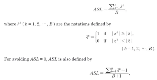
, G=D3-]D1+D2g Gb Db Db Db 3 1 2 = -_ + i ( b = 1, 2, ··· , B ). 　Then we have the achieved significance level ASL:

, ASL B b B b 1m =

!

= where mb_{( b = 1, 2, ··· , B ) are the notations defined by}

if if , G G G G 1 0 b b b₁ $ m =* ( b = 1, 2, ··· , B ). For avoiding ASL = 0, ASL is also defined by

ASL B 1 1 b B b 1m = + + =

!

when

!

bB=1mb1f ( f is a sufficiently small positive number). We can say that the null hypothesis H0 ( two samples X1 and X2 have common probability distributions: U1 = U2 ) is rejected if ASL is less than or equal to the significance level.

Application to psychophysical threshold estimates

(i) Mathematical notations and definitions

　Let X be the set of binomial observations:

, , , , .

X="xj nj]j=1 2 g Ng,

Let Xi ( i = 1, 2, ··· , n ) be the properly chosen intervals of the explanatory variable and let xri ( i = 1, 2, ··· ,

n ) be the mid-point of Xi. We assume that n ≤ N. Then we define the following notations:

if if , x x 1 0 ij j j i i g ! d X X =* ( i = 1, 2, ··· , n ; j = 1, 2, ··· , N ), and , , , , . ni ij mi ij j i 1 2 n j N j N 1 1 g d d n = = = = = ] g

!

(7)

Psychophysical Threshold Estimates 64 1047700_川崎英文誌17巻2号_2校_佐藤 By CS3<P64>　 We note thatN ni. i n 1 = =

!

　Let p xt] g=p_x; a b ct t, , 0i be the probability given by optimal parameters at, bt and c0 such that , p x =p x0 +c0 1-p x0 t] g t ] g ] t ] gg . exp p x0 = +1 - -a bx -1 t ] g _ _ t t ii

　We define the psychophysical threshold p with guessing rate c0

. p 2 1 1 0 p=_t- _d +c _n

(ii) The visual acuity test of the two-sample problem

　Since we adopt the Landolt-C of four different orientations in our visual acuity test, the guessing rate c0 is chosen as

c0 = 0.25.

　The explanatory variable x in our measurement is the logarithmic visual acuity.

　Let X1 (sample 1) and X2 (sample 2) be samples from the populations which have possibly different probability distributions U1 and U2 respectively. We shall test the following hypothesis:

null hypothesis H0 : U1 = U2, alternative hypothesis H1 : U1 ≠ U2.

　We took the data from 1 individual with no visual abnormalities in order to assess our bootstrap algorithm. The LogVA (Logarithmic Visual Acuity) is 0.3681 ± 0.0209 in complete refractive correction and we adopt this data set as sample 1. The data of sample 2 is taken in +0.50D incomplete refractive correction from the same individual of sample 1.

　Table 1 and Table 2 show the observed data of sample 1 ( N1 = 120 ) and sample 2 ( N2 = 80 ) respectively. Table 3 shows sample 3 ( N3 = 200 ) which is constructed by the combined data of samples 1 and 2.

　The logistic regression results of samples 1, 2 and 3 are shown in Table 4. Figures 1, 2, and 3 show the observed data and p xt] g=p_x; a b ct t, , 0i of samples 1, 2 and 3 respectively. Psychophysical thresholds pt ( k k

= 1, 2, 3 ) at probability = ( 1 + c0 ) / 2 = 0.625 are shown in Table 4.

　Now we shall prove that the samples 1 and 2 are taken from the populations which have different distributions.

Table 1 Observed data of sample 1　　　　　　　　Table 2 Observed data of sample 2 1047700_川崎英文誌17巻2号_2校_佐藤 By CS3<P63>　

Table 1: Observed data of sample 1 i x¯i ni mi mi/ni 1 0.156975 0 0 -2 0.198368 20 19 0.95 3 0.244125 20 18 0.9 4 0.295278 20 18 0.9 5 0.353270 20 13 0.65 6 0.420216 20 8 0.4 7 0.499398 20 8 0.4 N1= 7 � i=1 ni= 120 14

Table 2: Observed data of sample 2 i ¯xi ni mi mi/ni 1 0.156975 13 9 0.6923 2 0.198368 14 12 0.8571 3 0.244125 13 12 0.9231 4 0.295278 13 5 0.3846 5 0.353270 13 2 0.1538 6 0.420216 14 3 0.2143 7 0.499398 0 0 -N2= 7 � i=1 ni= 80 15

(8)

Table 3 Observed data of sample 3　　　　Table 4 Logistic regression results of samples 1, 2 and 3

Fig. 1 Observed data and p xt] g=p_x; a b ct t, , 0i of sample 1

Fig. 2 Observed data and p xt] g=p_x; a b ct t, , 0i of sample 2

Fig. 3 Observed data and p xt] g=p_x; a b ct t, , 0i of sample 3 Table 3: Observed data of sample 3

i ¯xi ni mi mi/ni 1 0.156975 13 9 0.6923 2 0.198368 34 31 0.9118 3 0.244125 33 30 0.9091 4 0.295278 33 23 0.6970 5 0.353270 33 15 0.4545 6 0.420216 34 11 0.3235 7 0.499398 20 8 0.4 N3= 7 � i=1 ni= 200 16

Table 4: Logistic regression results of samples 1, 2 and 3 sample 1 (k = 1) sample 2 (k = 2) sample 3 (k = 3)

Nk 120 80 200 ˆ αk 6.2105 4.5209 4.4349 ˆ βk -16.8720 -18.3394 -14.1192 γ0 0.25 0.25 0.25 se(ˆαk) 1.4383 1.5872 0.9012 se( ˆβk) 4.2411 6.6365 3.0423 se(γ0) 0.0 0.0 0.0 ˆ ξk 0.3681 0.2465 0.3141 se( ˆξk) 0.0209 0.0214 0.0170 Dk 115.546 90.241 224.026 G = D3− (D1+ D2) = 18.239 17 1.00 0.75 0.50 0.25 0.0 0.1 0.2 0.3 0.4 0.5 0.6 p x

Figure 1: Observed data and ˆp(x) = p(x; ˆα, ˆβ, γ0) of sample 1

20 1.00 0.75 0.50 0.25 0.0 0.1 0.2 0.3 0.4 0.5 0.6 p x

21 1.00 0.75 0.50 0.25 0.0 0.1 0.2 0.3 0.4 0.5 0.6 p x

(9)

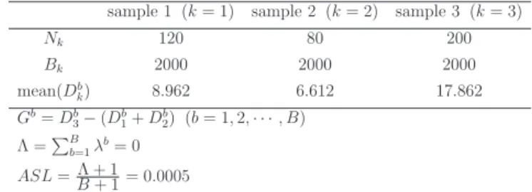
　The results of non-parametric bootstrap resampling are shown in Table 5. Since K b B

b

1m

= =

_

!

i is small for B = 2000, ASL is obtained as

1 . . ASL B K 1 0 0005 = + + =

This ASL shows that H0 is rejected at a very small significant level.

Table 5 Two-sample test by bootstrap resampling

(iii) The visual acuity test of one-sample problem

　We use the same example described in (ii). We shall test here the parameters a, b and threshold p by using bootstrap resampling. Since the methods of one-sample test for a, b and p are the same, we show here only the case of p.

　We adopt the following hypothesis:

null hypothesis H0 : p = pc,

alternative hypothesis H1 : p ≠ pc,

where pc is a prescribed value (which may be chosen from the threshold of control sample). Let pt and se

(pt) be the threshold and its standard error respectively of the (original) logistic regression. Let zt be the test statistics defined by se . z c p p p = -t t t _ i

Let pb_{( b = 1, 2, ··· , B ) be the thresholds obtained by the logistic regression of each bootstrap resampling.}

Let pr be the mean of pb_{( b = 1, 2, ··· , B ) :}

. B 1 b B 1 p= p = b r

_!

Let se(p) be the standard error of pb_{( b = 1, 2, ··· , B ) :}

. se B 2 1 b B 2 1 p p p = - = -b r ] g

_!

] g

Then we have the bootstrap test statistics zb_{( b = 1, 2, ··· , B ) as}

se .

zb b

p

p p

= -r_{] g}

Table 5: Two-sample test by bootstrap resampling sample 1 (k = 1) sample 2 (k = 2) sample 3 (k = 3)

Nk 120 80 200 Bk 2000 2000 2000 mean(Db k) 8.962 6.612 17.862 Gb_{= D}b 3− (D b 1+ D b 2) (b = 1, 2, · · · , B) Λ =�B b=1λ b_{= 0} ASL = Λ + 1_{B + 1 = 0.0005} 18

(10)

We have the achieved significance level ASL:

, ASL B b B b 1m =

!

= where mb_{( b = 1, 2, ··· , B ) are the notations defined by}

if if , z z 1 0 b b b ₁ ; ; ; ; m = ;z ;$; ;tz t * ( b = 1, 2, ··· , B ). For avoiding ASL = 0, ASL is also defined by

, ASL B 1 1 b B b 1m = + + =

!

when

!

bB=1mb1f ( f is a sufficiently small positive number). We can say that the null hypothesis H0 ( p =

pc) is rejected if ASL is less than or equal to the significance level.

　In the cases of one-sample tests of a and b, we adopt the following hypothesis:

null hypothesis H0 : a = 0, alternative hypothesis H1 : a ≠ 0, for a, and null hypothesis H0 : b = 0, alternative hypothesis H1 : b ≠ 0, for b.

　One-sample tests by bootstrap resampling for a, b, p in samples 1, 2 are shown in Table 6.

Table 6 One-sample test by bootstrap resampling Table 6: One-sample test by bootstrap resampling

sample 1 (k = 1) sample 2 (k = 2) Nk 120 80 Bk 2000 2000 ˆ αk 6.2105 4.5209 ASL∗1 k 0.0005 0.0050 ˆ βk -16.8720 -18.3394 ASL∗2 k 0.0005 0.0095 ˆ ξk 0.3681 0.2465 ASL∗3 k - 0.0005 min I0.95 0.355 0.231 max I0.95 0.380 0.262 ∗1_H 0: αk= 0, H1: αk�= 0 (k = 1, 2) ∗2_H 0: βk= 0, H1: βk�= 0 (k = 1, 2) ∗3_H 0: ξ2= ξ1, H1: ξ2�= ξ1 Λk= �Bk b=1λb (k = 1, 2) ASLk= Λ_Bk+ 1 k+ 1 19

(11)

(iv) Confidence interval of threshold

　The symbols of pt, se(pt), pb_{( b = 1, 2, ··· , B ), pr and se(p) are the same as in (iii).}

　Let } (z) be the cumulative distribution function of bootstrap resampling defined by

, }z B z z 1 b b B 1 31 1 3 { = - + = ] g

!

] g ] g

where {b _{(z) ( b = 1, 2, ··· , B ) are functions of z :}

z1z if if , z 1 z z 0 b b b $ { ] g=* ( b = 1, 2, ··· , B ).

We note that } (z) satisfies

, }]zg"0 ]z"-3g

. }]zg"1 ]z"+3g

Then we can obtain the confidence interval It of confidence coefficient t ( 0 < t < 1 ) such that

: } se } se . I 2 1 2 1 1 _$ _{# #} 1 _$ p- -t p p p+ +t p t t - d n ] g t - d n ] g

The confidence intervals I0.95 of threshold p for samples 1 and 2 are shown in Table 6.

Concluding remarks

　We proposed the bootstrap resampling algorithm for the psychophysical threshold estimates. Main properties of our algorithm are summarized in the following:

(i) the logistic regression including the guessing rate,

(ii) the non-parametric bootstrap resampling with log-likelihood ratio statistics for two-sample testing, (iii) the non-parametric bootstrap resampling for one-sample testing to certify the values of parameters and threshold obtained by logistic regression.

　We applied our bootstrap algorithm to the visual acuity test problem. Our algorithm does not require the identity of the number of observations between two samples. We can say that the bootstrap resampling provides a useful tool which has the flexibility of sampling in actual visual acuity measurements.

Acknowledgements

　The authors are very grateful to the referees for their very helpful comments.

References

1. Efron B, Tibshirani RJ: An Introduction to the Bootstrap. Boca Raton, Chapman & Hall / CRC, 1993.

2. Davison AC, Hinkley DV: Bootstrap Methods and their Application. New York, Cambridge University Press, 1977.

3. Foster DH, Bischof WF: Bootstrap estimates of statistical accuracy of thresholds obtained from psychometric functions. Spatial Vision 11: 135-139, 1997.

(12)

4. Foster DH, Bischof WF: Thresholds from psychometric functions: Superiority of bootstrap to incremental and probit estimators. Psychol Bull 109: 152-159, 1991.

5. Joy S, Chatterjee S: A bootstrap test using maximum likelihood ratio statistics to check the similarity of two 3-dimensionally oriented data samples. Math Geology 30: 275-284, 1998.

6. Good PI: Resampling Methods, A Practical Guide to Data Analysis. Boston, Birkh¨auser, 2006.

7. Nagai T, Hoshino T, Uchikawa K: Statistical significance testing of thresholds estimated by constant stimuli method. Vision 18: 113-123, 2006. (in Japanese).

8. Bach M: The Freiburg visual acuity test-automatic measurement of visual acuity. Optom Vis Sci 73: 49-53, 1996.

9. Beck RW, Moke PS, Turpin AH, Ferris FL 3rd, SanGiovanni JP, Johnson CA, Birch EE, Chandler DL, Cox TA, Blair RC, Kraker RT: A computerized method of visual acuity testing: Adaptation of the Early Treatment of Diabetic Retinopathy Study testing protocol. Am J Ophthalmol 135: 194-205, 2003.

10. Schulze-Bonsel K, Feltgen N, Burau H, Hansen L,Bach M: Visual acuities “hand motion” and “counting fingers” can be quatified with the Freiburg visual acuity test. Invest Ophthalmol Vis Sci 47: 1236-1240, 2006.

11. Mita N, Hara H, Kani K, Tabuchi A: Use of statistical analysis for visual acuity measurement. Jpn J of Vis Sci 31: 19-25, 2010 (in Japanese).

12. McCullagh P, Nelder JA: Generalized Linear Models. London, Chapman & Hall, 1989. 13. Christensen R: Log-Linear Models and Logistic Regression. New York, Springer, 1997. 14. Harrell FE Jr: Regression Medeling Strategies. New York, Springer, 2001.