Spatial Structure of Tokyo Metropolitan Area
Tawhid MONZUR 1Abstract
This research is focused on analyzing the urban spatial structure of the Tokyo Metropolitan Area (TMA) by using the Exploratory Spatial Data Analysis (ESDA) approach. To address the main research objective, the spatial structure of the population is analyzed. For this research Global Moran’s I and Local Moran’s I were selected. The population Census data 2000 is used for this analysis. ArcGIS 10.1 and GeoDa software are used to project and analyze the population census data. Population numbers are converted to density to exclude the influence of the census unit area sizes. The analysis pointed out specific locations of clustering types by proving the existence of spatial association and heterogeneity and differences in the case of the spatial pattern of population distribution.
Keywords: Exploratory spatial data analysis (ESDA), GIS, Population, Spatial structure, Tokyo
Metropolitan Area (TMA)
Introduction
Studying urban spatial structure, especially that of large urban areas, is becoming more important than ever because of the current pace of urban growth. The Current pace of population growth is considered as a “problem of the many” in the environment, social, and economic domain, which needs proper policies and planning initiatives for urban regeneration in a sustainable manner (Smith 2011; Knaap et al 2013; Bertaud 2001, 2004; Rode et al 2008; Lee 2007; Glaeser and Khan 2001; Mieszkowski and Mills 1993).
This research has selected Tokyo for analysis. Firstly, the urban management plan of Tokyo is praised because of its uniqueness and effectiveness (Hein, 2010). Secondly, the urban development process of Tokyo experienced multiple political, economic, and environmental upheavals, but still carries fame for attaining a sustainable urban form (Cho 2011; Morita et al 2012). Thirdly, to understand the overall spatial structure of TMA by using the ESDA approach, and assess its suitability in studying a large area. Henceforth, understanding spatial structure of TMA could contribute to both Tokyo and the emerging Asian cities in urban and regional planning. Asia Pacific countries are facing a problem of proper urban planning. Besides, most of the metropolitan areas located in the Asia Pacific are beset with social, environmental and economic issues referred to as the “The developing country phenomena” (Bugliarello 1999). New emerging cities in the Asia Pacific region are more complex in nature and difficult to study by using the conventional methods of urban studies. This research has selected a group of spatial statistical approaches simply called the Exploratory Spatial Data Analysis (ESDA) that has been effectively used for urban structure analysis from 2 perspectives: (1) the first group of research studied the Employment distribution2 (e.g., Baumont et al 2004; Guillain et al 2006), and (2) the second group of research studied the Population distribution3 (e.g., Millward and Bunting 2008; Millward 2008)
The research is constructed to study the spatial structure of TMA by using the ESDA approach. To address the research goal, the spatial structure of the population is analyzed because population is sensitive to changes in urban structure (Baum-Snow 2007). The research uses the Geographic Information System (GIS) and applies the Exploratory Spatial data analysis (ESDA) approach. Moreover, this research will also explore methods to observe the suitability of this approach in studying the spatial structure of the Tokyo Metropolitan Area.
1 Graduate School of Asia Pacific Studies, Ritsumeikan Asia Pacific University, Beppu, Oita, Japan. E-mail:
2 Employment distribution studied for the urban areas are- Los Angeles, The United States, eight departments of
Ile-de-France region, Ile-de-France, Singapore, Singapore, the Jakarta Metropolitan Area (JMA), Indonesia, Alexandria, Egypt, Rome, Italy, Athens, Greece, Hermosillo, Mexico and Dijon, France.
The paper is structured as follows. The next section is a brief review of theoretical and empirical studies that have been done for studying Tokyo’s spatial structure, as well as methods that have been applied. The 3rd section describes the study area, data collection, and preparation for the analysis, with the description of a spatial weight matrix. Section 4 deals with the methods of explanation and the empirical results. Finally, the conclusion describes the research findings and further analysis that can improve the research results.
2. Urban Spatial Structure Studied for Tokyo
The spatial structure of Tokyo has been studied from different perspectives. It has been analyzed based on a historical review, categorization of important events, location and amenities preferences, and employment distribution and inter-urban population distribution/migration (for example, see, Ichikawa 1994; Watanabe 1972, Watanabe et al 1980; Kikuchi and Obara 2004; Sorensen 2001a, 2001b; Okata and Murayama 2011; Pernice 2007; Tonuma 1998; Hein 2010). Tokyo has a good transportation network, which connects the urban and suburban locations, and enables the city population to commute from long distances. Decentralization, as stated in the paper of An (2008), is one of the main governmental policies which has been emphasized for reducing the concentration within the CBD (Central Business District) areas. To get rid of the negative urban externalities, government plans seemed successful for the development of the CBD areas but some research studies have criticized the idea of concentration outside the CBD areas that worsen the situation of suburbanization, which became one of the prominent issues that the government of Tokyo has had to deal with (Sorensen 2001a, 2004). Several urban policies have been implemented, but population concentration surpasses all the regulations.
Tokyo spatial structure studies can be found in papers where the main focus was on personal income, transportation costs, land price fluctuations, and land use changes for agricultural purposes that influenced the spatial pattern of Tokyo (Fujita and Kashiwadani 1989; Zheng 1990, 1991; Inoue et al 2007; Kikuchi and Obara 2004). A Local Moran’s I with k-order neighbors was used to analyze the distribution of elderly people in Ichikawa City (Zhang and Murayama 2011), and selected only a small part of TMA.
Articles related to the Tokyo spatial structure are large in number and focused on modeling the factors that affect distribution, and lack of a visual understanding. Only a very small number of research has actually tried to understand the spatial structure itself. They failed, however, to study the whole metropolitan region. This research looks at the overall spatial structure of TMA by looking at the differences in the distribution of population and that can fill the gaps of spatial structure studies previously done for studying TMA. By further research, the spatial structure of TMA can contribute to better urban policy-making for the region, and serve as a reference to the emerging megacities of the Asia Pacific region in urban planning and policy implementation (Uchiyama and Okabe 2012).
This research has selected the spatial statistical approach in analyzing the spatial structure of TMA because past research studies have used a regression based approach, cluster approach, or Grid-based approach in studying the spatial structure of TMA (for example, see Alpkokin et al 2007; Zheng 1991; Bagan and Yamagata 2012). A statistical based approach, however, was used by Zhao and Murayama (2005) to analyze the land use pattern focused on a small part of the central business district (CBD) in the TMA. In contrast, this research tends to analyze the spatial structure of the TMA on a regional level. The next section describes the study area and methods used for this research.
3. Research Approach and Methodology
This research selected the GISA (Global Indicator of Spatial Association) and LISA (Local Indicator of Spatial Association), the two branches of ESDA approach in studying the spatial structure of TMA used by many small and large cities to understand spatial association and spatial heterogeneity in spatial structure, which are lacking in the cases studying the TMA.
3.1 Tokyo Metropolitan Area
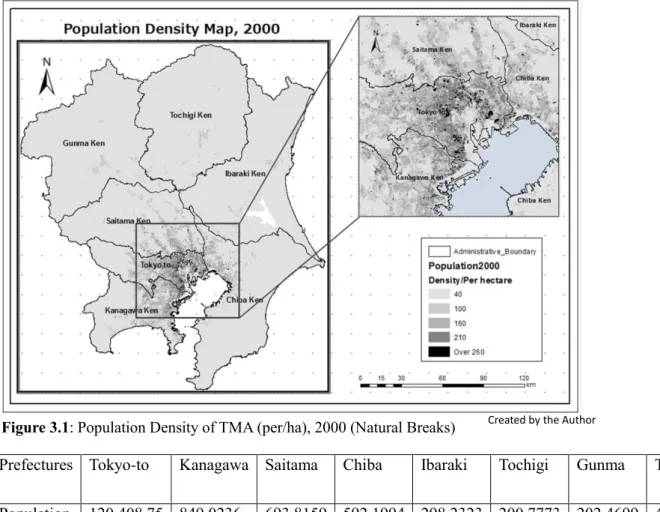
This research focuses on the Tokyo Metropolitan Area, including the 23 inner wards and the neighboring prefectures: Saitama, Kanagawa, Chiba, Gumma, Ibaraki, and Tochigi. It is an area of 32,028〖km〗^2 and is referred to as the largest mega metropolitan region in the world. Tokyo shares 8.5% of the land in Japan and has a population of 40.4 million people, mostly concentrated around the Tokyo Metropolitan Area (based on the 2000 census data). It is the economic hub of Japan, with a high rate of population concentration. (Table 1).
Figure 3.1: Population Density of TMA (per/ha), 2000 (Natural Breaks)
Prefectures Tokyo-to Kanagawa Saitama Chiba Ibaraki Tochigi Gunma Total Population 120,408,75 849,0236 693,8159 592,1994 298,2323 200,7773 202,4699 404,060,59 Household 541,3504 334,1301 248,2408 217,1144 984,814 668,352 695,058 157,565,81
Table 1: Demographic distribution in Tokyo Metropolitan Area, 2000 (Source: Authors calculation
from the employment dataset
3.2 Data
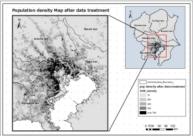
This research uses population census data from 2000, collected from the Ministry of Internal Affairs and Communications (MIC). The population census dataset contains different sets of variables, but for this research, only the population distribution data has been manipulated by using Excel’s statistical software. The boundaries of the census area units are provided in an ArcGIS shapefile as presented in Figure 3.1. Since the areas of census units (polygons) are different, this study further divided the study area into 200 meter by 200-meter cells, with the population evenly allocated to each cell according to the total population
number within the polygon. It contains 804,002 cells in total. From Figure 3.2, it can be observed that after treating the density dataset, the locations of high density are clearly visible.
Conceptual representation of the location is a prerequisite in order to identify the spatial association and spatial heterogeneity (Baumont et al 2004; Guillain et al 2006). A Spatial Weight Matrix is constructed based on the notion that each observed value is linked to a set of adjacent neighboring observed values, which is exogenous by nature (Baumont et al 2004). The elements of the weight matrix (w_ii) have 0 diagonals whereas the elements (w_ij=1) represent the spatial influence of location i to location j. For this research, Queens contiguity weight matrix (1st order) has been selected with at least 9 conjoined cells, and are considered a clustered location (Getis and Aldstadt 2002).
Figure 3.2: Population density Map after data treatment, 2000
For the tabulation and manipulation of the extracted data, Excel statistical software is used. Also, the spatial statistical toolsets are analyzed by using the ArcGIS 10.1 and GeoDa software.
4. Empirical Results
4.1 Global Moran’s I
The Global Moran’s I, also called the Global Spatial Autocorrelation, measures the linearity of the observed value to its neighboring values, which determine the identification of the spatial distribution patterns (Dispersed, Random and Clustered) of a certain phenomenon (Goodchild 1986, Griffith 1992)
To determine the spatial patterns Global Moran’s I provide two sets of Moran’s I indexes; Positive Moran’s I Index and Negative Moran’s I Index. The 3rd set of indexes appears when the Moran’s I Index provides 0 (ArcGIS resource)4.
The dispersed spatial pattern means that each observed value from its neighboring values is located far from each other, or has less linearity between the observed value and the neighboring values. In this case,
4http://resources.esri.com/help/9.3/arcgisengine/java/gp_toolref/spatial_statistics_tools/how_spatial_autocorrelation_col
on_moran_s_i_spatial_statistics_works.htm
Moran’s I index will be negative. The Random spatial pattern means the distribution of the values is independent. More precisely, no spatial connection existed between the observed and neighboring values (Moran’s I Index will be 0). The Clustered spatial pattern means most of the values are concentrated in nearby locations or adjacent together, and Moran’s I index will be positive. Moran’s I can be written as follows (Viton 2010): 𝐼 = ( 𝑆 ∑ 𝑖𝑗 𝑤𝑖𝑗) ∑ 𝑖𝑗 𝑤𝑖𝑗 (𝑏𝑖−𝑏̅)(𝑏𝑗−𝑏̅) ∑ 𝑖(𝑏𝑖−𝑏̅)2 Where, S = number of observations
∑ 𝑖𝑗 𝑤𝑖𝑗 = sum over all i and j of 𝑤𝑖𝑗 𝑤𝑖𝑗 = spatial weight between i and j. 𝑊𝑖𝑗 (𝑏𝑖𝑏𝑗) = weight * cross product terms.
The Global Moran’s I analysis output (Moran’s I index is 0.93) reveals that a strong spatial autocorrelation exists within the population distribution in TMA. More precisely, the Global Moran’s I Index proves that the distribution of the population in Tokyo tends to have a clustered spatial pattern. Moreover, The Z-score is as high as 1662.85 while higher than +2.58 can show enough that there is a 99% chance that the data is taking a clustered pattern (ArcGIS resource)5.
Global Moran’s I analysis gives an overall result of the formation of a certain type of spatial pattern in the selected area. However, Global Moran's I analysis alone cannotprovide enough evidence to identify the spatial differences. The output failed to provideevidence about the locations of high and low values. To find out the high and low-density locations and also the dissimilar locations, Local Moran’s I is used and discussed in the next section.
4.2 Local Moran’s I
The Global Moran’s I analysis, found strong evidence that a clustered pattern exists in TMA in terms of population distribution, but fails to identify what type of clustering and the locations of the spatial association and spatial heterogeneity. On the other hand, Local Moran’s I calculates each location separately (different locations of an area). Local Moran’s I is technically a localized version of Global Moran’s I that looks at the specific locations and provides evidence on the assumption of the Global Moran’s I. The Local Moran’s I identify the significant locations of positive or negative autocorrelation. The Local Moran’s I can be written as follows (Anselin 1995)-
𝐼𝑖 = 𝑏𝑖∑ 𝑤̂𝑖𝑗 𝑏𝑗 𝑗 Where, 𝑏𝑖 = 𝑍(𝑏𝑖) =𝑏𝑖𝜎−𝑏̅ & [𝜎 =∑ (𝑏𝑖−𝑏̅) 2 𝑗 𝑠−1 ]
The Local Moran’s I analysis divides all the values into five separate groups based on the Local Moran’s I Index and the significance level. Local Moran’s I not only identifies the high and low values but also addresses the outliers of the values. Insignificant (i.e. no significant clustering exists); High-High group (i.e. high values are clustering with other neighboring high values and are above the mean); Low-Low group (i.e. low values are clustering with other low values and below the mean); High-Low group (i.e. high values clustering with low values and are below the mean); and Low-High group (i.e. low values are clustering with high values and are below the mean). The first 2 groups (HH and LL) signify a positive spatial autocorrelation or, in other word, spatial clustering. The 3rd and 4th group (HL and LH) signify a negative spatial autocorrelation, or are what is known as outliers or dissimilar values (Baumont, et al 2004; Anselin 1995).
5http://resources.esri.com/help/9.3/arcgisdesktop/com/gp_toolref/Spatial_Statistics_toolbox/what_is_a_z_score_what_is
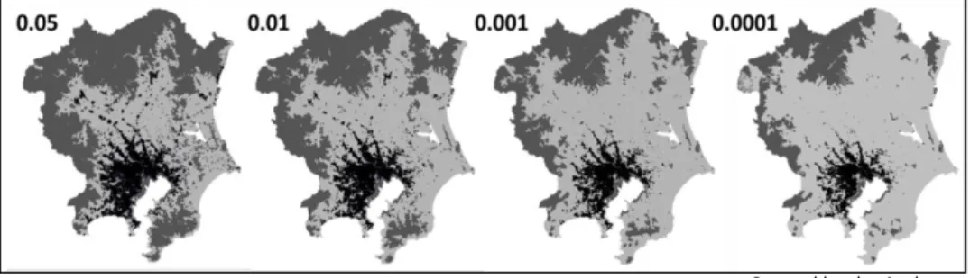
Figure 4.1 shows the 5 types of clustering in TMA. The insignificant clustering or NS group pattern contains the highest number of 364,295 cells, the High-High clustering group or pattern contains about 82,474 cells, Low-Low clustering group or pattern contains 356,163 cells, Low-High clustering group or pattern contains 1057 cells and high-low clustering group or pattern contains 2 cells. The outcome provided by the Local Moran’s I calculation are statistically significant at a 0.05 confidence level. Interpretation of the outputs and identification of the locations of 5 clustering types is very difficult at a 0.05 level of significance, or is too general. In this case, threshold significance levels are selected (0.01, 0.001 and 0.0001 level of significance) to observe the clustering types. From figure 4.2, the differences in spatial clustering can be visible in cases of population distribution, which selected locations as clusters based on the intensity of the clustering
Figure 4.1: The 5 types of Clustering (at 0.05 Level of Significance)
The Local Moran’s I analysis identified the specific locations of the high-density areas or hotspots and low-density areas or cold spots in TMA. Besides, the analysis also identified the outliers or dissimilar locations mostly adjacent to high population density areas.
Figure 4.2: The 5 Clustering types at 0.05, 0.01, 0.001 and 0.0001 Level Of Significance.
5. Conclusion
This paper contributes to urban spatial structure studies through using the ESDA statistical approach in studying the spatial structure of the Tokyo Metropolitan Area. For this research, a population distribution dataset for the year 2000 was selected and analyzed. Global Moran’s I and Local Moran’s I were used for this research.
This research selected a widely used statistical based approach, ESDA, to study a large urban area, in this case the TMA. The ESDA approach has been used to study the spatial structure of many large and small cities, and proved effective and easy to use. In the case of the TMA, Local Moran's I analysis identified the locations of high and low clustering as well as outliers/dissimilar locations, providing an explanation for the spatial structure of the TMA to a great extent. The difference between the previous methods and ESDA is, ESDA addressed the locations of the high and low clustering as well as intensity of the clustering that previous research papers lacked in studying the spatial structure of TMA. Moreover, ESDA based studies in case of employment and population distribution studied the differences in locations or looked at one cluster type to draw a conclusion. This research used ESDA in a different way to understand the spatial structure where the threshold significance level is considered as classifying further the cluster types to different ranked centers to see the incite of the spatial pattern.
Spatial structure of population distribution: the Local Moran’s I analysis, identified the locations of high and low density as well as identified the locations of dissimilar areas in case of population distribution in TMA. In general, The Local Moran’s I analysis separated all values into 5 different clustering types based on a 0.05 level of significance and showed all potential locations of clustering. To identify the true locations of clustering, threshold significance levels were selected (0.01, 0.001 and 0.0001 level of significance) that identified the locations based on the intensity of the relations between the observed and neighboring values that Global Moran’s I indexes failed to provide. The intensity of the clusters can further help to analyze the centers and sub-centers of the TMA as well as employment distribution.
For this research, I have used a grid of 200X200m^2, but it could be different if the size of the grids is changed. Further studies will look at the differences in grid size and their impact over spatial pattern analysis. The research can be further improved by looking at land use changes over time based on population and employment distribution. Further research also aims to use population and employment variables to analyze what made the dissimilar clustering types exist within the TMA. Additionally, distribution of employment, transportation, and population for recent years will be studied to analyze the changes in the spatial pattern in the TMA.
The explained methods and findings of this research can help in spatial pattern studies of the Asia Pacific region. The emerging cities in the Asia Pacific region are going through an urban transformation, and it is necessary to understand the spatial structure both at the local and regional levels. Uchiyama and Okabe’s (2012) research paper visually showed the emerging cities transformation that could be problematic for the future of urban studies. Henceforth, this research can help provide a broader perspective in studying and analyzing the spatial pattern of emerging cities. Nonetheless, to understand the spatial structure of a city, it is
necessary to identify the differences in spatial patterns that can guide urban planners in decision-making and implementation of urban policies at a regional level.
Notes:
An abstract version of this paper is presented in 23rd GIS Association of Japan conference.
References
Alpkokin, Pelin., Komiyama, Naohisa., Takeshita, Hiroyuki, and Kato, Hirokazu. (2007).
Tokyo Metropolitan Area Employment Cluster Formation in Line with Its Extensive Rail Network. Journal of the Eastern Asia Society for Transportation Studies 7: 1403–1416.
Anselin, Luc. (1995). Local indicators of spatial association—LISA. Geographical analysis 27(2): 93-115.
An, Sang Kyung. (2008). Recentralization of Central Tokyo and Planning Responses. Journal of Regional Development Studies 11: 1-20.
Bagan, Hasi, and Yamagata, Yoshiki. 2012. Landsat analysis of urban growth: How Tokyo
became the world's largest megacity during the last 40 years. Remote sensing of Environment 127: 210-222.
Baumont, Catherine, Ertur, Cem, and Le Gallo, Julie. 2004. Spatial Analysis of Employment
and population Density: The Case of the Agglomeration of Dijon 1999. Geographical Analysis 36(2): 147-176.
Baum-Snow, Nathaniel. 2007. Suburbanization and transportation in the Monocentric model. Journal of Urban Economics 62: 405-423.
Bertaud, Alain. 2001. Metropolis: A measure of the spatial organization of 7 large cities. Unpublished working paper. Provide the source
Bertaud, Alain. 2004. The spatial organization of cities: Deliberate outcome or unforeseen
consequence? Institute of Urban and Regional Development. UC Berkeley: Institute of Urban and Regional Development. Provide the source
Bugliarello, George.1999. Megacities and the developing World. The bridge, 29(4):19-26. Cho, Seungyeou. 2011. Urban transformation of Seoul and Tokyo by local redevelopment
project. ITU A/Z 8(1): 169-183.
Fujita, Masahisa, and Kashiwadani, Masuo. 1989. Testing the Efficiency of Urban Spatial Growth: A Case Study of Tokyo. Journal of Urban Economics 25: 156-192.
Getis, Arthur and Aldstadt, Jared (2002). Constructing the Spatial Weights Matrix Using a Local Statistic. Geographical Analysis 34 (2): 130-140.
Glaeser, Edward L. and Kahn, Matthew E. 2001. Decentralized employment and the
transformation of the American city (No. w8117). National Bureau of Economic Research. Goodchild, Michael F. 1986. “Spatial Autocorrelation”. Norwich: Geo Book.
Griffith, Daniel A. 1992. What is spatial autocorrelation? Reflections on the past 25 years of spatial statistics. Espace géographique 21(3): 265-280.
Guillain, Rachel, Julie Le Gallo, and Boiteux-Orain, Celine. 2006. Changes in spatial and
Hein, Carola. 2010. Shaping Tokyo: Land Development and Planning Practice in the Early Modern Japanese Metropolis. Journal of Urban History 36(4): 447-484.
Ichikawa, Hiroo. 1994. The evolutionary process of urban form in Edo/Tokyo to 1900. The town planning review, 65(2): 179-196.
Inoue, Ryo, Kigoshi, Naoyuki, and Shimizu, Eihan 2007. “Visualization of spatial distribution
and Temporal change of land prices for residential use in Tokyo 23 wards using Spatio-Temporal Kriging.” Pp.1-11 in Proceedings of 10th international conference on computers in urban planning and urban management, 63. Tokyo.
Kikuchi, Toshio, and Obara, Norihiro. 2004. Saptio-temporal changes of urban fringe in Tokyo metropolitan area. Geographical reports of Tokyo metropolitan university 39: 57-69. Knaap, Gerrit-Jan, Lewis, Rebecca and Schindewolf, Jamie. 2014. The Spatial Structure of
Cities in the United States. 지리학논총 (Geography Journal) 60: 1-26.
Lee, Bumsoo. 2007. Edge and Edgeless cities? Urban spatial structure in US metropolitan areas. Journal of regional science 47(3): 479-515.
Morita, Tetsuo, Nakagawa, Yoshihide, Morimoto, Akinori, Maruyama, Masateru, and
Hosokawa, Yoshimi. 2012. Changes and Issues in Green Space Planning in the Tokyo Metropolitan Area: Focusing on the "Capital Region Plan". International Journal of Geomate 2(1): 191-196.
Mieszkowski, Peter, and Mills, Edwin S. 1993. The causes of Metropolitan Suburbanization. The Journal of Economic Perspectives 7(3): 135-147
Millward, Hugh and Bunting, Trudi. 2008. Patterning in urban population densities: a
spatiotemporal model compared with Toronto 1971-2001. Environment and Planning A 40: 283-302. Millward, Hugh. 2008. Evolution of Population Densities: Five Canadian Cities, 1971-2001.
Urban Geography 29(7):616-638.
Okata, Junichiro, and Murayama, Akito. 2011. “Tokyo’s Urban Growth, Urban Form and
Sustainability”. Pp.15-41 in Megacities: Urban Form, Governance, and Sustainability, eds. A. Sorensen and J. Okata. Tokyo: Springer Japan.
Pernice, Raffaele. 2007. Urban Sprawl in Postwar Japan and the Vision of the City based on the
Urban Theories of the Metabolists′. Journal of Asian Architecture and building Engineering 6(2): 237-244.
Rode, Philipp, Wagner, Julie, Brown, Richard, Chandra, Rit, Sundaresan, Jayaraj, Konstantinou,
Christos, Tesfay, Natznet and Shankar, Priya. 2008. Integrated city making Governance planning and transport (No. 25223). London School of Economics and Political Science, LSE Library, London: Urban age programme.
Smith, Duncan Alexander. 2011. “Polycentricity and Sustainable Urban Form: An Intra-Urban
Study of Accessibility, Employment and Travel Sustainability for the Strategic Planning of the London Region.” Doctoral dissertation, Centre for Advanced Spatial Analysis & Department of Geography, University College London.
Sorensen, André. 2001a. Building suburbs in Japan: continuous unplanned change on the urban fringe. TPR 72(3): 247-273.
Sorensen, André. 2001b. Subcenters and Satellite Cities: Tokyo’s 20th Century Experience of Planned Polycentrism. International Planning Studies 6(1): 9-32.
Sorensen, André. 2004. “Major issues of land management for sustainable urban regions in
Japan.” Pp. 197-216 in Towards Sustainable Cities: East Asian, north American and European Perspectives on managing Urban Regions, eds. A Sorensen, P J. Marcotullio and J. Grant. Hampshire: Ashgate publishing limited.
Tonuma, Koichi. 1998. Tokyo: Policies toward the 21st century. Ekistics 65: 388-390. Uchiyama, Yuta and Okabe, Akiko. 2012. Categorization of 48 Mega-Regions by Spatial
Patterns of Population Distribution: The Relationship between Spatial Patterns and Population Change. 48th ISOCARP International Planning congress. (2012, 09, 10-2012, 09, 13) Perm, Russia.
Viton, Philip A. 2010. Notes on Spatial Econometric Models. City and Regional Planning 870(3): 2-17.
Watanabe, Yoshio. 1972. Some aspects of recent Japanese metropolitan growth. Geographical reports of Tokyo metropolitan university 6/7: 51-62.
Watanabe, Yoshio, Takeuchi, Kazuhiko, Nakabayashi, Itsuki and Kobayashi, Akira. 1980.
Urban growth and landscape change in the Tokyo metropolitan area. Geographical Reports of Tokyo metropolitan University 14/15: 1-26.
Zhang, Changping and Murayama, Yuji. 2011. “Testing local spatial Autocorrelation using
k-order neighbors”. Pp.45-56 in Spatial Analysis and Modeling in Geographical Transformation Process: GIS-based application, eds. Y. Murayama and R. B. Thapa. London: Springer.
Zheng, Xiao-Ping. 1990. The spatial Structure of Hierarchical inter-urban system: equilibrium and optimum. Journal of Regional Science 30(3): 375-392.
Zheng, Xiao-Ping. 1991. Metropolitan Spatial Structure and its Determinants: A Case-study of Tokyo. Urban Studies 28(1): 87-104.
Zhao, Yaolong and Murayama, Yuji. (2005). Effect characteristics of spatial resolution on the
analysis of urban land-use pattern: a case study of CBD in Tokyo using spatial autocorrelation index. Pp.585-594 in Cities in Global Perspective: Diversity and Transition, eds. Y Murayma and G Du. Tokyo: College of Tourism, Rikkyo University with IGU Commision.