Parallel Imports, Drug Price Control and
Pharmaceutical Innovation
journal or
publication title
Discussion paper series
number
26
page range
1-29
year
2005-08-05
DISCUSSION PAPER SERIES
Discussion paper No.26
Parallel Imports, Drag Price Control
and Pharmaceutical Innovation
Ken Tabata
Kobe City University of Foreign Studies Tetsuya Shinkai
,Kwansei Gakuin University Satoru Tanaka
Kobe City University of Foreign Studies and
Makoto Okamura ,Hiroshima University
August 2005
SCHOOL OF ECONOMICS
KWANSEI GAKUIN UNIVERSITY
1-155 Uegahara Ichiban-cho Nishinomiya 662-8501, Japan
Parallel Imports, Drug Price Control and
Pharmaceutical Innovation
Ken Tabata
∗Tetsuya Shinkai
†Satoru Tanaka
‡Makoto Okamura
§August 5, 2005
Abstract
This paper examines how parallel importation influences pharma-ceutical innovation and the welfare of the economy, when crossnational drug price differentials occur not only because of demand elasticity based factors, but also governmental drug price control based factors. By explicitly considering the governmental drug price control based factors, this paper shows that parallel importation may enhance phar-maceutical innovation, when the bargaining power of a foreign gov-ernment is strong and the price elasticity of demand in the foreign market is small. We also show that the increase in R&D induced by parallel imports may even increase the consumer surplus of a country with high demand elasticities and which could face relatively low drug prices, if parallel imports were not allowed.
Keywords: Parallel Imports, Pharmaceutical Innovation, Drug Price Control JEL classification: F13: I18: L65
∗Corresponding author. Address: Kobe City University of Foreign Studies, 9-1,
Gakuenhigashimachi,Nishi-ku, Kobe, 651-2187, Japan; E-mail: [email protected]
†Kwansei Gakuin University
‡Kobe City University of Foreign Studies §Hiroshima University
1
Introduction
Recently, many economists have argued that high income countries should prohibit parallel imports of drugs from low income countries (e.g. Kremer, 2002 and Danzon et al, 2003). A ban on parallel imports enables a phar-maceutical company to set different prices in different markets according to price elasticities of demand (“demand elasticity based price differentials”). Since demand elasticities are inversely related to income, the profit maximiz-ing pharmaceutical company sets lower (higher) drug prices in lower (higher) income countries. Thus, a ban on parallel imports improves access to the medicine in low income countries while it provides a greater incentive for a product development to the pharmaceutical company, since it can allow companies to capture closer to the full social surplus for their product.
These arguments implicitly assume that the crossnational drug price dif-ferentials are mainly due to demand elasticity based factors. However, em-pirical studies, such as that of Maskus (2001) and Scherer (2003), show that there are many other complicated factors that explain observed crossnational drug price differentials. In particular, governmental price control for phar-maceutical products is known to be one of these crucial factors. Moreover, it is also known that the form and extent of governmental price controls are heavily influenced by the lobbying activities of pharmaceutical companies. That is, the negotiation process between pharmaceutical companies and the government. Therefore, suppose the crossnational drug price differentials are mainly due to factors based on governmental price control; then, it is not self evident that the ban on parallel imports of drugs really leads to increased pharmaceutical innovation.
Focusing upon factors based on governmental price control in crossna-tional drug price differentials, Pecorino (2002) reexamines the impact of par-allel imports upon a pharmaceutical company’s profits and R&D incentives. In his model, one monopolist in the home country sells in both the domestic and foreign markets. Since these two markets have identical demand elastici-ties, the demand elasticity based price differentials never occur. The firm can freely set its domestic price. However, owing to governmental price control, the foreign price is determined by the Nash bargaining game between the firm and the foreign government. In the No Reimport regime (NR regime), the domestic government does not allow parallel imports of drugs. Thus, perfect market segmentation is possible and the firm charges its profit maximiz-ing price in the domestic market while the negotiated foreign price becomes lower than in the domestic market. Therefore, under the NR regime, the price differentials are purely due to factors based on the governmental price control (“price control based price differentials”). In the Reimport regime
(R regime), the domestic government allows parallel imports of drugs. Thus, the law of one price holds and the negotiated foreign price also becomes the domestic price as well (“uniform pricing effect”). This fact implies that the negotiation results influence not only the profits from the foreign market, but also the profits from the domestic markets under the R regime. Therefore, a firm has an incentive to bargain harder under the R regime than under the NR regime (“strengthened negotiation effect”).
The comparison of the results under the NR regime and the R regime sug-gests that parallel imports may provide the following two competing impacts upon the firm’s profits and R&D incentives. First, parallel importation has a negative impact upon the firm’s total profits through the “uniform pricing effect” since it lowers the domestic price and the profits from the domestic market. However, second, parallel importation has a positive impact upon the firm’s total profits through the “strengthened negotiation effect” since it increases the level of the uniform price in both the domestic and foreign markets. Pecorino (2002) shows that the latter “strengthened negotiation effect” always dominates the former “uniform pricing effect” under the plau-sible specification of the demand function. Thus, parallel importation has positive impacts upon the pharmaceutical company’s profits and incentives to invest in R&D.
These existing studies show that, if the differential pricing is purely de-mand elasticity based, parallel importation reduces pharmaceutical innova-tion. However, if the differential pricing is based on purely governmental price control, parallel importation promotes pharmaceutical innovation. There-fore, the purpose of this paper is to construct a theoretical model that en-ables us to analyze the cases where price differentials occur because of both demand elasticities and negotiation based factors. Then, we analyze more extensively under what economic environments parallel importation leads to increased or decreased pharmaceutical innovation. Moreover, by explicitly considering the existence of the price control based price differential, we re-examine the impact of parallel importation upon the consumer surplus of the home and foreign country. Since the observed crossnational price differ-entials are due to various complicated factors, including both governmental price control based and demand elasticity based factors, it is significant to investigate these issues carefully for the sake of more valuable policy debates. This paper extends the model by Pecorino (2002) in the following two ways. First, we consider the case where each domestic and foreign market has different price elasticities of demand, which enables us to analyze the case where the price differentials occur because of both demand elasticity and negotiation based factors. Second, we explicitly formulate a firm’s decisions about R&D investment, which is not explicitly analyzed in Pecorino (2002).
Based upon these two extensions, this paper shows that parallel imports may enhance pharmaceutical innovation when the bargaining power of the foreign government is strong and the price elasticity of demand in the foreign market is small. We also show that this increase in R&D induced by parallel imports may even increase the consumer surplus of the foreign country. The possibility of the foreign consumer surplus improving because of the parallel imports has not been considered rigorously in previous literature.
The structure of the paper is as follows. Section 2 establishes the basic setup. Section 3 examines the case where the domestic government does not allow parallel imports (NR regime). Section 4 examines the case where the domestic government allows parallel imports (R regime). Section 5 examines the impact of parallel imports upon R&D investment by comparing the re-sults from the NR regime and the R regime. Section 6 examines the impact of parallel imports upon welfare. Section 7 presents our conclusions.
2
Basic Setup
Following Pecorino (2002), this paper considers a simple partial equilibrium model of trade that consists of two countries: home (H) and Foreign (F). A firm in the home country produces a good of quality s > 0, which can be thought of as a pharmaceutical product sold in both the domestic and foreign markets. We use a model of vertical product differentiation to represent consumer preferences in each market. Consumers differ in their tastes for the product quality, but they rank quality in the same way. When a consumer of type t in the market i = H, F buys a product of quality s at a price pi, his or her utility is given by ui = ts− pi. If a consumer does not buy, his or her outside option is normalized to zero. In each market i, a consumer of type t is uniformly distributed between 0 and Ti with unit density. For clarity of the analysis, we consider the case TF ≤ TH and specify TH and
TF as follows: TH = T and TF = φT 0 ≤ φ ≤ 1. These specifications assume that the maximum willingness to pay in the foreign market is smaller than or equal to that in the domestic market. After a simple calculation, it also implies that the price elasticities of demand in the foreign market are larger than or equal to those in the domestic market. Therefore, as the value of φ becomes larger and approaches one, the value of the price elasticities of demand in the foreign market becomes smaller and approaches the value in the domestic market. Conversely, as the value of φ becomes smaller, the value of the price elasticities of demand in the foreign market becomes larger
relative to that in the domestic market.1
A firm conducts R&D and sets the quality of its product according to a cost function C(s), which satisfies C′(s) > 0 and C′′(s) > 0. Then, it manufactures and delivers its product in both the domestic and foreign mar-kets. Once a product has been developed, its marginal cost of production is not affected by the level of quality. Thus, we normalize the marginal cost of production to zero. If the domestic government provides no reimport regime (NR regime), reimports of the good back into the home country are not al-lowed. Thus, a firm can set a different price in each market because perfect market segmentation is possible under the NR regime. However, if the do-mestic government provides a reimport regime (R regime), reimportation of the good back into the home country is allowed. Thus, a firm has to set a uniform price for both the domestic and foreign markets.
Therefore, the order of decision making is summarized as follows. First, the domestic government declares a parallel import regime. Then, the firm decides on the quality levels with which it will endow its product. Finally, the firm manufactures and delivers the product in each market and sets the prices. In the following subsections, we examine the quality and price determination process in both the N R and R regimes.
3
NR Regime
We first consider the price determination process under the assumption that costs of quality development have already been sunk. Since perfect market segmentation is possible under the NR regime, a firm can set different prices in each market. In the domestic market, since the firm has patent protection on this product, it can act as a monopolist. Since t is uniformly distributed between 0 and TH, the demand in the home country is XH(pH) = sT−ps H. Thus, the profit on domestic sales is given by ΠH(pH) = sT−pH
s p
H. By maximizing this profit with pH, we obtain
pHN R(s) = sT
2 , (1)
ΠHN R(s) = (sT )
2
4s , (2)
1The price elasticities of demand in the domestic market ϵ
H and in the foreign market
ϵF are expressed as follows: ϵH = sTp−p and ϵF = sφTp−p. Therefore, a lower value of φ
implies a higher value of the price elasticities of demand in the foreign market relative to the domestic market.
where pHN R(s) is the price and ΠHN R(s) is the profit in the domestic market under the NR regime. In order to stress that these values depend upon the level of product quality s, we denote them as a function of s.
The demand and the profit in the foreign market are given by XF(pF) = sφT−pF
s and Π
F(pF) = sφT−pF
s p
F. If the firm were free to set its own price in the foreign market, it would charge the monopoly price sφT2 and obtain the profit (sφT )4s 2. However, because of governmental control of the drug price, the foreign drug price is determined by the Nash bargaining game between the firm and the foreign government. This assumption is relevant in the pharmaceutical context.
The foreign government would like to maximize consumer surplus in its country, whereas the monopolist would like to maximize profits from sales in the foreign market. The consumer surplus in the foreign country is given by CSF(pF) = (sφT2s−pF)2. In the absence of agreement, profits and consumer surplus are both zero. Thus, zero is the threat point for both the domestic firm and the foreign government. Therefore, the Nash bargained price in the foreign market under the NR regime pFN R is found by maximizing
[CSF(pF)]α[ΠF(pF)]1−α, (3) with pF subject to the condition that Π(pF) ≥ 0 and CSF(pF) ≥ 0. Here,
α reflects the bargaining power of the foreign country. A simple calculation
yields pFN R(s) = (1− α)sφT 2 , (4) ΠFN R(s) = (1− α 2)(sφT )2 4s , (5) where pF
N R(s) is the price and ΠFN R(s) are the profits in the foreign market under the NR regime. The results here depend very obviously on α. When
α = 1, since the foreign government has the all the bargaining power, we
must have pF
N R(s) = 0 and ΠFN R(s) = 0, which means that profit for sales in the foreign market is zero. On the other hand, when α = 0, since the domestic firm has the all the bargaining power, we have pF
N R(s) = sφT
2 and
ΠFN R(s) = (sφT )4s 2, which means that the domestic firm charges the monopoly price and obtains monopoly profit in the foreign market.
Under the NR regime, total profits of firms from sales in both the domestic and foreign markets, which are given by ΠT otalN R (s) = ΠHN R(s) + ΠFN R(s), are
ΠT otalN R (s) = (sT )
2
4s [1 + (1− α
Moreover, the consumer surplus of the home country CSN RH (s), which is given by (sT−PN RH (s))2
2s and the consumer surplus of the foreign country CS
F N R(s) , which is given by (sφT−PN RF (s))2 2s , are as follows. CSN RH (s) = (sT ) 2 8s , (7) CSN RF (s) = (sφT ) 2 8s (1 + α) 2. (8)
Finally, the social surplus of the home country SSN RH (s), which is given by the sum of the total profits of domestic firm ΠT otal
N R (s) and consumer surplus of home CSH
N R(s), is ΠT otalN R (s) + CSN RH (s).
Then, we consider the quality choice of the firm. The firm will choose its quality level s in order to maximize its net total profit under the NR regime
ˆ
ΠN R(s):
ˆ
ΠN R(s) = ΠT otalN R (s)− C(s). (9) The first order condition to this problem implies
C′(s) = Π T otal N R (s) s , = T 2 4 [1 + (1− α 2)φ2]. (10)
Let the quality level that solves Equation (10) be denoted as sN R, which ex-presses the level of the R&D investment conducted by a firm under the NR regime. Therefore, by substituting this sN R into Equations (1), (4),(6),(7) and (8), we can obtain the value of prices in both the domestic and for-eign markets, consumer and social surpluses of the home country, and the consumer surplus of the foreign country under the NR regime.
4
R Regime
We first consider the price determination process. Under the R regime, the negotiated foreign price also becomes the domestic price, owing to the ability to reimport and the absence of transportation costs. Thus, the law of one price holds for the good in question: (i.e. pH = pF = p).
The foreign drug price is again determined by the negotiation between the firm and the foreign government. The foreign government’s surplus from bargaining under the R regime is CSF(p) and the threat point is zero, which is analogous to the NR regime case. However, the domestic firm’s surplus
(threat point) changes from ΠF(pF) (0)under the NR regime to ΠH(p) + ΠF(p)−ΠH
N R(s) (ΠHN R(s) ) under the R regime. ΠH(p)+ΠF(p) reflects profits in both the domestic and foreign markets when reimports are allowed, and ΠHN R(s) only reflects the profits from sales in the domestic market achieved by setting the home country monopoly price sT2 .
These changes in the firm’s surplus and the threat points are explained as follows. Under the NR regime, whether or not agreement is reached, profits from home sales are always ΠH
N R(s). Therefore, the firm’s surplus from bargaining is independent of the profits from home sales. However, under the R regime, the firm’s profit from home sales is influenced by the negotiated foreign price. As a result, the term ΠH(p) appears in the firm’s surplus. In the absence of agreement, the firm cannot sell in the foreign market. However, the firm can at least obtain profits ΠHN R(s) by setting monopoly price sT2 in the home country. Therefore, the threat point of firms under the R regime becomes ΠH
N R(s). This implies that, if the condition ΠH(p) + ΠF(p)≥ ΠHN R(s) (11) does not hold, the firm does not sell in the foreign market. Taking this constraint into account, we obtain the following Lemma.
Lemma 1 .
If the price elasticities of demand in the foreign market relative to in the domestic market are sufficiently high to satisfy the condition that φ < √2− 1, there exists no incentive for firms to sell in the foreign
market under the R regime.
The proof is shown in Appendix A. When the price elasticities of demand in the foreign market are sufficiently high to satisfy the condition that φ <
√
2− 1, a firm would have to set a sufficiently low uniform price under the R regime if the drug were sold in both the domestic and foreign markets. However, the profits obtained from sales in both the domestic and foreign markets under such a low uniform price are smaller than the profit obtained by selling only in the domestic market ΠH
N R(s) at the home monopoly price. Thus, with the R regime, when φ <√2− 1, the firm sets its price as follows.
pR1(s) =
sT
2 , (12)
where pR1(s) denotes the price under the R regime when φ <
√
2−1. In addi-tion, the total profits under the R regime, which are given by [sT−psR1(s)]pR1(s), are
ΠT otalR1 (s) = (sT )
2
where ΠT otalR1 (s) denotes the profit under the R regime when φ < √2− 1. Since pR1(s) = pHN R(s) holds by definition, the condition ΠT otalR1 (s) = ΠHN R(s) also holds.
Suppose the condition φ ≥ √2− 1 holds, the domestic firm reaches an agreement with the foreign government and starts to sell in the foreign mar-ket. Thus, when φ≥√2− 1, the Nash bargained uniform price under the R regime is found by maximizing
[CSF(p)]α[ΠH(p) + ΠF(p)− ΠHN R(s)]1−α, (14) with p subject to the condition that CSF(p) ≥ 0 and Equation (11). Here, Equation (11) is rewritten as ˜ p≤ p ≤ ¯p. (15) where ˜ p≡ sT 4 [1 + φ− p (1 + φ)2− 2], and ¯ p≡ sT 4 [1 + φ + p (1 + φ)2 − 2].
Taking this constraint into accounts, we obtain
pR2(s) = sT 8 [(1 + α)(1 + φ) + 4(1− α)φ − √ X], (16) where X ≡ (1 + α)2(1 + φ)2− 8[α + (1 − α)2φ(1− φ)]
and pR2(s) denotes the price under the R regime, when φ ≥
√
2− 1. In addition, when φ ≥ √2− 1, the total profits Πtotal
R (s) under the R regime, which is given by [sT−psR2(s)]pR2(s) + [sφT−psR2(s)]pR2(s), are
ΠT otalR2 (s) = (sT ) 2 4s Y, (17) where Y ≡ [(1− α 2)(1 + φ)2 4 + 2(1− α) 2φ(1 − φ) + α +(1− α)(3φ − 1) 4 √ X] and ΠT otal
R2 (s) denotes the profits under the R regime when φ ≥
√
2− 1. Appendix B explains the deduction of Equation (16) more rigorously. The results here again depend very obviously on α. When α = 1, since the foreign government has the all the bargaining power, we must have PR2(s) = ˜p, which
is the lowest price satisfying the participation constraints of the domestic firm. On the other hand, when α = 0, since the domestic firm has the all the bargaining power, we have PR2(s) = sT4 (1 + φ), which is the monopoly price that maximizes ΠH(p) + ΠF(p) given the restriction on uniform pricing under the R regime.
The changes in the domestic firm’s surplus and the threat points discussed above suggest that price concessions by the firm under the R regime are much more costly than those under the NR regime, because they affect the domestic market as well as the foreign market. As a result, we should expect the domestic firm to drive a harder bargain under the R regime than under the NR regime. We denote this as the “strengthened negotiation effect” due to the parallel imports. This “strengthened negotiation effect” leads to higher total profits under the R regime than under the NR regime. Therefore, the condition ΠT otal
R (s)≥ ΠT otalN R (s) f or∀ s is more likely to hold. However, under the R regime, the law of one price holds because of the ability to reimport. We denote this as the “uniform pricing effect” due to the parallel imports. This “uniform pricing effect” leads to lower profits under the R regime than under the NR regime. Therefore, the condition that ΠT otal
R (s) ≥ ΠT otalN R (s) f or ∀ s is less likely to hold. Thus, the overall effect on firm profitability appears to be ambiguous.
Therefore, under the R regime, the price PR(s) and the total profits of firm ΠT otalR (s) are expressed as follows.
PR(s) ½ = PR1(s) if φ < √ 2− 1, = PR2(s) if φ ≥ √ 2− 1, (18) ΠT otalR (s) ½ = ΠT otal R1 (s) if φ < √ 2− 1, = ΠT otal R2 (s) if φ≥ √ 2− 1. (19) Moreover, the consumer surplus of the home country CSH
R(s), which is given by (sT−P2sR(s))2, is CSRH(s) ½ = CSH R1(s) if φ < √ 2− 1, = CSR2H (s) if φ≥√2− 1, (20) where CSR1H (s) ≡ (sT ) 2 8s , CSR2H (s) ≡ (sT ) 2 128s[7− 5φ + α(3φ − 1) + √ X]2.
Here, CSH R1(s) ≡ (sT−PR1(s))2 2s and CS H R2(s) ≡ (sT−PR2(s))2 2s . In addition, the
consumer surplus of the foreign country CSF
R(s), which is given by (sφT−PR(s))2 2s , is CSRF(s) ½ = 0 if φ <√2− 1 = CSR2F (s) if φ≥√2− 1 (21) where CSR2F (s)≡ (sT ) 2 128s[(1 + α)(3φ− 1) + √ X]2. Here, CSF R2(s)≡ (sφT−PR2(s))2
2s and the consumer surplus in the foreign market
becomes zero, since the firm does not sell in the foreign market when φ <
√
2−1. Finally, the social surplus of the home country SSH
R(s), which is given by the sum of the total profits of domestic firm ΠT otal
R (s) and the consumer surplus of the home country CSRH(s), are ΠT otalR (s) + CSRH(s).
Then, we consider the quality choice of the firm. The firm will choose its quality level s in order to maximize its net total profit under the R regime
ˆ ΠR(s):
ˆ
ΠR(s) = ΠT otalR (s)− C(s). (22) The first order conditions to this problem imply
C′(s) = Π T otal R (s) s , ½ = T2 4 if φ < √ 2− 1, = T42Y if φ≥√2− 1. (23)
Let the quality level that solves Equation (23) be denoted as sR1(sR2), which expresses the level of the R&D investment conducted by a firm under the R regime, when φ <√2− 1 (φ ≥√2− 1). Therefore, by substituting these sR1 and sR2 into Equations (12), (13),(16),(17),(20) and (21), we can obtain the values of the price, consumer surplus and social surplus of the home country, as well as the consumer surplus of the foreign country under the R regime.
5
The Impacts of Parallel Imports upon R&D
investment and the Net Total Profit
This section examines how parallel importation influences R&D investment and the net profit of the firm. By comparing the results in Equation (10) and (23), we obtain the following proposition
1. When the price elasticities of demand in the foreign market are suf-ficiently high to satisfy the condition that φ < √2− 1, the relation ΠT otal
R (s)≤ ΠT otalN R (s) f or ∀ s holds. Thus, the R&D investment under
the NR regime is higher than or equal to that under the R regime. 2. When the price elasticities of demand in the foreign market are
suffi-ciently low to satisfy the condition that φ≥√2− 1,
(a) the R&D investment under the NR regime is higher than or equal to that under the R regime, if the relation ΠT otal
R (s)≤ ΠT otalN R (s) f or∀ s
holds.
(b) the R&D investment under the R regime is higher than or equal to that under the NR regime, if the relation ΠT otalR (s)≥ ΠT otalN R (s) f or∀ s
holds.
The proof is shown in Appendix C. Proposition 1-1 indicates that parallel importation leads to lower R&D investment, if the price elasticities of demand in the foreign market are sufficiently high to satisfy the condition that φ <
√
2− 1. When φ < √2− 1, under the R regime, the firm has no incentive to sell in the foreign market as shown in Lemma 1. Thus, the firm sells only in the domestic market at the home monopoly price and obtains profits ΠT otal
R1 (s) = ΠHN R(s). However, under the NR regime, the firm has an incentive to sell in both the domestic and foreign markets irrespective of the value of φ, since the firm can set different prices in different markets according to their price elasticities of demand. Thus, the firm sets the price PH
N R(s) in the home country and PN RF (s) in the foreign country, respectively, and obtains profits ΠT otal
N R (s) = ΠHN R(s) + ΠFN R(s). These results suggest that parallel importation makes it impossible for the firm to obtain profits from the foreign market, when φ < √2− 1 (“the loss of foreign market effect”). Thus, parallel importation leads to lower R&D investment when φ < √2− 1 because of “the loss of foreign market effect”.
However, Proposition 1-2 indicates that parallel importation may lead to higher R&D investment if the price elasticities of demand in the foreign market are sufficiently low to satisfy the condition that φ≥√2− 1 and the condition ΠT otalR (s) ≥ ΠT otalN R (s) f or ∀ s holds. As mentioned in the Section 4, since the negotiated foreign price affects not only the profits from the foreign market, but also the profits from the domestic market, the firm has an incentive to drive a harder bargain under the R regime than under the NR regime. This “strengthened negotiation effect” leads to higher total profits under the R regime than under the NR regime. Therefore, the condition ΠT otalR (s) ≥ ΠT otalN R (s) f or ∀ s is more likely to hold. However, under the R
regime, the law of one price holds because of the ability to reimport. This “uniform pricing effect” leads to lower profits under the R regime than under the NR regime. Therefore, the condition that ΠT otal
R (s)≥ ΠT otalN R (s) f or ∀ s is less likely to hold. These results suggest that parallel importation leads to higher R&D investment when φ ≥ √2− 1, supposing the “strengthened negotiation effect” dominates the “uniform pricing effect”.
To investigate more extensively under what economic environments for parallel importation leads to higher or lower R&D investment, we compare the results under the NR and R regimes for some values of α and φ. Firstly, we examine the case when α = 0 and 1 and obtain the following results.
Result 1 .
1. When all the bargaining power resides with the domestic firm (α = 0), the R&D investment under the NR regime is higher than or equal to that under the R regime.
2. When all the bargaining power resides with the foreign government (α =
1), the R&D investment is the same under either regime.
The proof is shown in the Appendix D. Result 1-1 indicates that parallel importation leads to lower R&D investment when α = 0. When α = 0, since all the bargaining power lies with the domestic firm, price controls by the foreign government become meaningless. Thus, the firm can freely set the price in the foreign market under either the NR or R regime. Under the NR regime, the firm can set different prices in different markets. However, under the R regime, the firm has to set a uniform price in both markets. Thus, total profits under the R regime are lower than those under the NR regime.2 This result implies that parallel importation leads to lower firm profits and, thus, lower R&D investment. Note that, when α = 0, all the bargaining power lies with domestic firms irrespective of the parallel import regimes. Thus, the impact of the firm’s strengthened bargaining power induced by parallel importation becomes negligible. Therefore, the “uniform pricing effect” dominates the “strengthened negotiation effect”.
Result 1-2 indicates that parallel importation has no impact upon R&D investment when α = 1. When α = 1, since all the bargaining power lies with the foreign government, the foreign government can freely set the price in the foreign market under either the NR or R regimes. Under the NR regime, the foreign government maximizes the consumer surplus by setting
2The situation examined here when α = 0 is the same as the situation examined in the well-known models of third degree price discrimination such as those of Varian (1985) and Malueg and Schwartz (1994).
the foreign price as zero. Thus, the domestic firm obtains zero profits from sales in the foreign market. This means that the total profits under the NR regime equal the domestic monopoly profits (i.e. ΠT otal
N R (s) = ΠHN R(s)). However, under the R regime, the foreign government has to set the price that satisfies the participation constraint of the domestic firm defined in Equation (11). Thus, the firm sets the foreign price as ˜p, which is also becomes the
domestic price. From Equation (11), when p = ˜p, total profits under the
R regime equal the domestic monopoly profits (i.e. ΠT otal
R (s) = ΠHN R(s)). These results imply that parallel importation has no influence upon the firm’s profits and thus none on the R&D incentives. Note that, when α = 1, all the bargaining power lies with the foreign government irrespective of the parallel import regimes. Thus, the impact of the firm’s strengthened bargaining power induced by parallel importation becomes significant. Result 1-2 implies that the “strengthened negotiation effect” is large enough to cancel out the “uniform pricing effect”.
Secondly, we examine the case when φ = 12 and 1, respectively, and obtain the following results.
Result 2 .
1. When the price elasticities of demand in the foreign market satisfy the condition that φ = 12, the R&D investment under the NR regime is higher than or equal to that under the R regime.
2. When the price elasticities of demand in the foreign market satisfy the condition that φ = 1, R&D investment under the R regime is higher than or equal to that under the NR regime.
The proof is shown in the Appendix E. Results 2-1 and 2-2 indicate that parallel importation leads to lower R&D investment when φ = 12, whereas it leads to higher R&D investment when φ = 1. The higher value of φ implies a lower value of the price elasticities of demand in the foreign market. Therefore, the negative impacts of the “uniform pricing effect” weaken as the value of φ becomes higher.
When φ = 12, the price elasticities of demand in the foreign market are high enough. Thus, the “uniform pricing effect” dominates the “strengthened negotiation effect”. When φ = 1, the price elasticities of demand in the foreign market are low enough and equal to those in the domestic market. Thus, the “strengthened negotiation effect” dominates the “uniform pricing effect”.3
3The situation examined here when φ = 1 is the same as the situation examined in Pecorino(2002).
Finally, we consider the case when φ = 34 and 78, respectively, and obtain the following results.
Result 3 .
1. When the price elasticities of demand in the foreign market satisfy the condition that φ = 34, the R&D investment under the R regime is higher (lower) than or equal to that under the NR regime, if α ≥ ˆαφ=3
4 (α ≤
ˆ
αφ=3
4). The ˆαφ= 3
4 is defined as α, which satisfies the condition that
fφ=3 4(α) = 0, where fφ= 3 4(α)≡ 5 √ 25 + 18α + 25α2− (11α + 27).
2. When the price elasticities of demand in the foreign market satisfy the condition that φ = 78, the R&D investment under the R regime is higher (lower) than or equal to that under the NR regime, if α ≥ ˆαφ=7
8 (α ≤
ˆ
αφ=7
8). The ˆαφ= 7
8 is defined as α, which satisfies the condition that
fφ=7 8(α) = 0, where fφ= 7 8(α)≡ 13 √ 169 + 50α + 169α2− (27α + 171). 3. The value of ˆαφ=7
8 is smaller than the value of ˆαφ= 3 4.
The proof is shown in Appendix F . Results 3-1 and 3-2 indicate that, given a sufficiently high value of φ, parallel importation leads to the higher (lower) R&D investment, when the value of α is higher (lower) than a certain thresh-old value. Moreover, Result 3-3 provides us an insight that the range of α where the parallel import leads to higher R&D investment becomes wider as the value of φ becomes larger. Therefore, Result 3 suggests that parallel importation is likely to induce higher R&D investment, as the values of both
α and φ become larger.
The intuition behind these results is analogous to those in Results 1 and 2. The participation constraints of the firm defined in Equation (11) is the key driving force that causes the firm to bargain harder under the R regime than under the NR regime. The influence of these participation constraints become more prominent when the value of α is high and the bargaining power of the foreign government is strong. Consequently, given a sufficiently high value of φ, the “strengthened negotiation effect” is likely to dominate the “uniform pricing effect”, as the value of α becomes larger. In addition, as discussed in Result 2, a higher value of φ leads to a smaller impact of the “uniform pricing effect”. Therefore, a higher value of φ lowers the threshold value of α and widens the range of α where the “strengthened negotiation effect” dominates the “uniform pricing effect”.
In order to confirm the results discussed above and obtain more insight, we provide a numerical example. For illustrative purposes, we specify the
functional form of the cost function of R&D C(s) as
C(s) = 1 βs
β β > 1, (24)
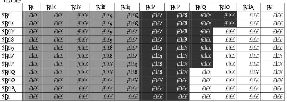
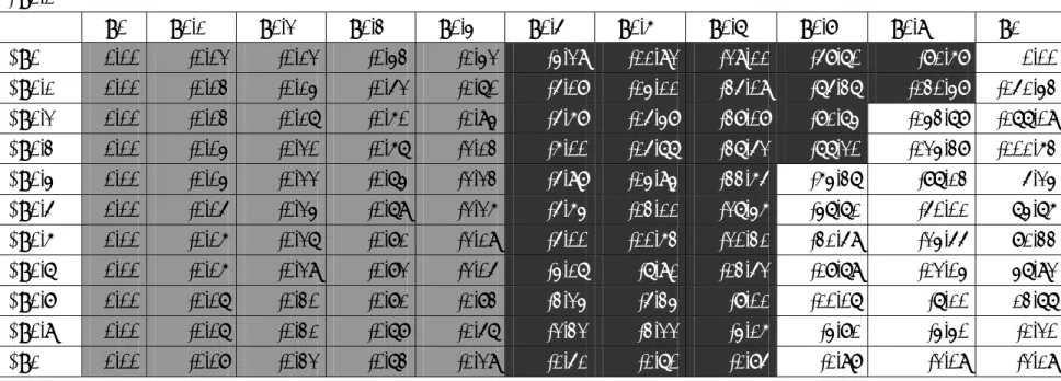
where β is the parameter that determines the curvature of the marginal cost function. A higher value of β implies a higher slope of the marginal cost function. Following Valletti (2005), we set the baseline parameterization of the model as follows: T = 10, k = 30 and β = 3. Then, given these values, we increase the values of φ and α from 0 to 1 in increments of 0.1.
Table 1 shows the difference in the R&D investment SR− SN R between the two regimes for various sets of the values of φ and α. For later analysis, we denote the parameter region of (φ, α) that satisfies φ≤ 0.4 < √2− 1 as the Case 1 region. The Case 1 region is shown as the shaded area in the light gray in Table 1. As shown in Proposition 1, when φ≤ 0.4 <√2− 1, parallel importation leads to lower R&D investment. In this region, since the price elasticities of demand in the foreign market are too high for the firm to sell in the foreign market under the R regime, parallel importation reduces the firm’s profits and incentives to invest in R&D.
When φ ≥ 0.5 > √2− 1, there exist two different regions. One is the region where parallel importation leads to lower R&D investment. The other is the region where parallel importation leads to higher R&D investment. We denote the former region as the Case 2 region and the latter region as the Case 3 region. The Case 2 (Case 3) region is shown as the area shaded dark gray (as the area without shading) in Table 1. Then, we can easily confirm that the Case 3 region lies in the area where the values of φ and α are larger than those in the Case 2. As discussed in Results 1, 2 and 3, when the both values φ and α are smaller (Case 2), the “uniform pricing effect” is likely to dominate the “strengthened negotiation effect”. Thus, parallel importation leads to lower R&D investment. However, when the values of both φ and α are larger (Case 3), the “strengthened negotiation effect” is likely to dominate the “uniform pricing effect”. Thus, parallel importation leads to higher R&D investment.
Before concluding this section, we confirm the impact of parallel impor-tation upon the net total profit of the domestic firm by explicitly considering the differences in the level as well as the cost of R&D investment between the R and the NR regimes. From Proposition 1 and the definitions of the Case 1, Case 2 and Case 3 regions, we obtain the following proposition.
Proposition 2 .
investment between the R and the NR regimes are explicitly taken into account.
1. In the Case 1 and Case 2 regions, the net total profit of the domestic firm under the NR regime ˆΠN R(sN R) is larger than or equal to in that
under the R regime ˆΠR(sR).
2. In the Case 3 region, the net total profit of the domestic firm under the R regime ˆΠR(sR) is larger than or equal to that under the NR regime
ˆ
ΠN R(sN R).
The proof is shown in Appendix G. Proposition 2-1 indicates that parallel importation deteriorates the net total profits of the domestic firm in both the Case 1 and Case 2 regions, and Proposition 2-2 indicates that it improves the net total profits of the domestic firm in the Case 3 region. Since the “loss of foreign market effect” exists in the Case 1 region, or the “uniform pricing effect” dominates the “ strengthened negotiation effect” in the Case 2 region, parallel importation leads to lower profits for the firm. However, in the Case 3 region, the “strengthened negotiation effect” dominates the “uniform pricing effect”. Thus, parallel importation leads to the larger profits of the firm. Proposition 2-1 and 2-2 confirm that this intuition holds even if we explicitly consider the differences in the level as well as the cost of R&D investment between the R and the NR regimes.
6
Welfare Analysis
This section examines how parallel importation influences the consumer sur-plus of the home and the foreign countries. Parallel importation influences the consumer surplus in the following two different ways. First, it influences the consumer surplus through its impact upon the pricing regime (i.e. the uniform pricing regime or the differential pricing regime). We denote this as the “pricing regime effect”. Second, it influences the consumer surplus through its impact upon the level of R&D investment. We denote it as the “R&D investment effect”. For the clarity of the analysis, we first ignore the “R&D investment effect” and only examine how the “pricing regime effect” influences the consumer surplus of the home and the foreign country. By using the results in Equations (7), (8),(20) and (21), we obtain the following Lemma.
Suppose there is no change in R&D investment under either the R regime and NR regime
1. Then, when φ <√2− 1 (in the Case 1 region), the consumer surplus
of the home country is the same under either the NR-regime or the R-regime, while the consumer surplus of the foreign country under the R regime is lower than or equal to that under the NR regime.
2. Then, when φ ≥ √2 − 1 (in the Case 2 and Case 3 regions), the
consumer surplus of the home country with the R regime is higher than or equal to that with the NR regime, whereas the consumer surplus of the foreign country with the R regime is lower than or equal to that with the NR regime.
The proof is shown in Appendix H. Lemma 2-1 indicates that parallel impor-tation has no influence upon the consumer surplus of the home country in the Case 1 region, whereas it deteriorates the consumer surplus of the foreign country, if we ignore the “R&D investment effect”. When φ < √2− 1, as shown in Equations (1) and (12), parallel importation has no impact upon the pricing method in the domestic market. Thus, the consumer surplus of the home country also does not change. However, parallel importation in-duces the firm not to sell in the foreign market in the Case 1 region (“the loss of market effect”). Thus, it makes the consumer surplus of the foreign country become zero.
Lemma 2-2 indicates that parallel importation leads to higher (lower) consumer surplus of the home (foreign) country in the Case 2 and Case 3 re-gions, if we ignore the “R&D investment effect”. This result is consistent with the results obtained in the previous literature such as Malueg and Schwartz (1994) and Varian (1985). If we ignore the “R&D investment effect”, parallel importation leads to lower (higher) prices in the domestic (foreign) market. Thus, it leads to a higher (lower) consumer surplus in the home (foreign) country.
Then, by explicitly considering both the “pricing regime effect” and the “R&D investment effect”, we obtain the following proposition.
Proposition 3 .
Suppose the differences in the R&D investment between the R regime and the NR regime are explicitly taken into account.
1. Then, in the Case 1 region, the consumer surplus of the home (foreign) country under the R regime is lower than or equal to that under the NR regime.
2. Then, in the Case 2 region, the consumer surplus of the foreign country with the R regime is lower than or equal to that with the NR regime, while it is ambiguous whether the consumer surplus of the home country with the R regime is higher or lower than with the NR regime.
3. Then, in the Case 3 region, the consumer surplus of the home country with the R regime is higher than or equal to that with the NR regime, while it is ambiguous whether the consumer surplus of the foreign coun-try in the R regime is higher or lower than under the NR regime.
The proof is shown in Appendix I. Proposition 3-1 indicates that parallel importation deteriorates the consumer surplus of the home and the foreign country in the Case 1 region, if we consider the “R&D investment effect” explicitly. The Case 1 region is defined as the parameter region of (φ, α), which satisfies φ <√2− 1. In the Case 1 region, as discussed in Lemma 2-1, the “pricing regime effect” has no influence upon the consumer surplus of the home country. However, as shown in Table 1, parallel importation lowers R&D investment because of the “loss of foreign market effect”. This lowers R&D investment and induces reduced quality of the product. Thus, parallel importation deteriorates the consumer surplus of the home country through its negative impacts upon R&D investment. In addition, as discussed in Lemma 2-1, parallel importation induces the firm to not sell in the foreign market. Thus, it makes the consumer surplus of the foreign country become zero.
Proposition 3-2 indicates that parallel importation deteriorates the con-sumer surplus of the foreign country in the Case 2 region, whereas its impact upon the consumer surplus of the home country is ambiguous, if we consider the “R&D investment effect” explicitly. The Case 2 region is defined as the parameter region of (φ, α) where parallel importation lowers the R&D in-vestment when φ ≥ √2− 1, since the “uniform pricing effect” dominates the “strengthened negotiation effect”. Lower R&D investment means lower quality of the product. Moreover, Lemma 2-2 shows that the “pricing regime effect” deteriorates the consumer surplus of the foreign country. Thus, par-allel importation unambiguously deteriorates the consumer surplus of the foreign country. The lower R&D investment induced by parallel importation also has a negative impact upon the consumer surplus of the home coun-try. However, as shown in Lemma 2-2, the “pricing regime effect” provides positive impacts upon the consumer surplus of the home country. Thus, it is ambiguous whether parallel importation improves or deteriorates the consumer surplus of the home country.
Proposition 3-3 indicates that parallel importation improves the consumer surplus of the home country in the Case 3 region, whereas its impact upon
the consumer surplus of the foreign country is ambiguous, if we consider the “R&D investment effect” explicitly. The Case 3 region is defined as the parameter region of (φ, α) where parallel importation leads to higher R&D investment when φ ≥ √2 − 1, since the “strengthened negotiation effect” dominates the “uniform pricing effect”. The higher R&D investment means higher product quality. Moreover, Lemma 2-2 shows that the “pricing regime effect” improves the consumer surplus of the home country. Therefore, parallel imports unambiguously improve the consumer surplus of the foreign country. The higher R&D investment induced by the parallel import also has a positive impact upon the consumer surplus of the foreign country. However, as shown in Lemma 2-2, the “pricing regime effect” has a negative impact upon the consumer surplus of the foreign country. Thus, it is ambiguous whether parallel imports improve or deteriorate the consumer surplus of the foreign country.
By explicitly considering the “R&D investment effect”, we can observe the following two interesting results. Propositions 2-1 and 2-2 suggest that parallel importation may deteriorate not only the consumer surplus of the foreign country, but also the consumer surplus of the home country in the Case 1 and Case 2 regions because of its negative impact upon the R&D investment. Thus, in the Case 1 and Case 2 regions, as the negative impact of the parallel import upon the R&D investment increases, parallel importa-tion is more likely to deteriorate the consumer surplus of the home country. This possibility of home consumer surplus deterioration due to parallel im-portation is not examined rigorously in previous literature. Moreover, by explicitly considering the existence of the “price control based price differ-entials”, we can observe the Case 3 region where parallel importation leads to higher R&D investment. In the Case 3 region, as shown in Proposition 2-3, parallel importation may improve not only the consumer surplus of the home country, but also the consumer surplus of the foreign country because of its positive impact upon R&D investment. Thus, in the Case 3 region, as the positive impact of parallel importation upon R&D investment increases, parallel importation is more likely to improve the consumer surplus of the for-eign country. This possibility of forfor-eign consumer surplus improvement due to the parallel import is also not examined rigorously in previous literature. These considerations suggest that parallel importation is likely to dete-riorate (improve) the consumer surplus of the home country in the Case 2 region if its negative impact upon R&D investment increases (decreases). In addition, parallel importation is likely to improve (deteriorate) the consumer surplus of the foreign country in the Case 3 region, if its positive impact upon the R&D investment increases (decreases).
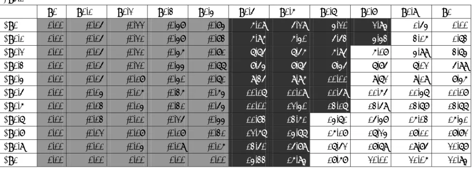
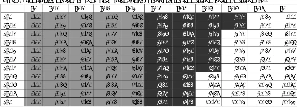
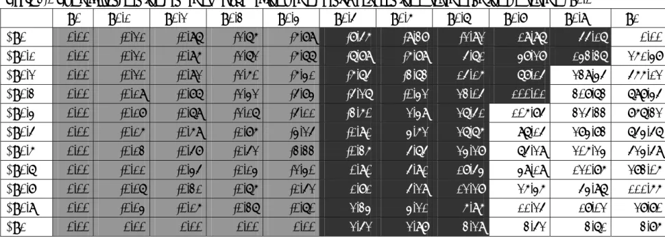
To confirm the result discussed above and obtain more insight, we again give a numerical example. Table 2-1 (Table 3-1) shows the difference in the consumer surplus of the home country CSH
R−CSN RH between the two regimes for various sets of the values of φ and α and Table 2-2 (Table 3-2) also shows the difference in the consumer surplus of the foreign country CSF
R − CSN RF . Again, the Case 1 region is shown as the light gray shaded area, the Case 2 region is shown as the dark gray shaded area, and the Case 3 region is expressed as the area without shading.
A lower value of β means a lower slope of the marginal cost function of the R&D investment. Simple calculation using Equations (10), (23) and (24) shows that a lower value of β induces larger differences in investments (|sR − sN R|) between the two regimes. Thus, as the value of β decreases, the “R&D investment effect” increases in all regions. Therefore, the negative (positive) impact of parallel imports upon the R&D investment becomes larger in the Case 2 region (the Case 3 region).
Tables 2-1 and 2-2 show the case where β is large (β = 3.1) and thus the “R&D investment effect” is small. As is consistent with the results in Proposition 2, we can confirm that parallel importation deteriorates the consumer surplus of both the home and foreign countries in the Case 1 region, deteriorates the consumer surplus of the foreign country in the Case 2 region, and improves the consumer surplus of the home country in the Case 3 region. Moreover, since β is large (β = 3.1) and the “R&D investment effect” is small, the “pricing regime effect” dominates the “ R&D investment effect”. Thus, we can confirm that parallel importation improves the consumer surplus of the home country in the Case 2 region, and deteriorates the consumer surplus of the foreign country.
On the other hand, Table 3 shows the case in which β is small (β = 1.1) and thus the “R&D investment effect” is large. In this case, the “ R&D investment effect” can dominate the “pricing regime effect”. Thus, we can find some regions where parallel importation deteriorates (improves) the consumer surplus of the home (foreign) country in the Case 2 region (the Case 3 region). Thus, when β is small (β = 1.1) and thus the “R&D investment effect” is large, in the Case 2 and 3 region, we can observe the somewhat counterintuitive impact of parallel trade.
7
Concluding Remarks
This paper examined how parallel importation influences pharmaceutical in-novation and the welfare of an economy, when the crossnational drug price differentials occur not only because of demand elasticity based factors, but
also because of factors based on governmental drug price control. This paper extended the model by Pecorino (2002) in the following two ways. First, we considered the case in which each domestic and foreign market had different price elasticities of demand. Second, we explicitly formulated the firm’s de-cisions about R&D investment. Based upon these two extensions, this paper showed that parallel importation might enhance pharmaceutical innovation when the bargaining power of the foreign government is strong and the price elasticity of demand in the foreign market is small. We also showed that this increase in R&D induced by parallel importation might even increase the consumer surplus of the foreign country. This possibility of foreign consumer surplus improvement due to parallel importation has not been considered rigorously in previous literature.
Recent policy debates on parallel importation of drugs have implicitly as-sumed that the crossnational drug price differentials occur because of demand elasticity based factors. However, in the drug price context, the governmental drug price control also plays a significant role. This paper showed that the qualitative impact of parallel importation upon pharmaceutical innovation and the welfare of the economy might differ substantially if factors based on governmental drug price control are considered explicitly. Therefore, for more valuable policy debates on the issue of the parallel import of drugs, we need to take much more care in considering the causes of crossnational drug price differentials.
Appendix A: Proof of Lemma 1
Since ΠH(p) + ΠF(p) = [(1+φ)sT−2p
s ]p, it is the quadratic function of p. Thus, ΠH(p) + ΠF(p) achieves its maximum value of (1+φ)8s2(sT )2 at p = (1+φ)sT4 . Therefore, the relation ΠH(p)+ΠF(p) ≥ ΠH
N R(s) does not hold, if
(1+φ)2(sT )2 8s <
ΠH
N R(s) =
(sT )2
4s . Simple calculation shows that this condition can be
rewrit-ten as (1 + φ)2 ≤ 2 or φ <√2− 1.
Appendix B: Deduction of Equation (16)
Let us define V (p)≡ [CSF(p)]α[ΠH(p)+ΠF(p)−ΠH
N R(s)]1−α. By maximizing Equation (14) with p subject to CSF(p) ≥ 0 and Equation (15), we obtain the following first and second order conditions, respectively:
Γ(p) ≡ αCS F ′(p) CSF(p) + (1− α) ΠT otal(p) ΠT otal′(p)− ΠH N R(s) = 0 (25)
Γ′(p) = −α 2 (sφT − p)2+(1−α) ΠT otal′′(p)(ΠT otal− ΠH N R(s))− (ΠT otal′(p))2 (ΠT otal(p)− ΠH N R(s))2 < 0 (26) where the right hand side of Equation (25) is defined as Γ(p).
After tedious calculation, Equation (25) is written as
4p2− [(1 + α)(1 + φ) + 4(1 − α)φ]sT p + [(1 − α)(1 + φ)φ + α 2](sT )
2 = 0.
Thus, we obtain the following two candidates for the optimal interior solution.
p1, p2 =
sT
8 [(1 + α)(1 + φ) + 4(1− α)φ ±
√ X].
Since 0≤ φ ≤ 1 and (1 + φ)2 ≥ 2 because of φ ≥√2− 1, we can show that
X = (1 + α)2(1 + φ)2− 8[α + (1 − α)2φ(1− φ)] ≥ 2(1 + α)2
− 8[α + (1 − α)2φ(1
− φ)]
= 2(1− α)2[1− 4φ(1 − φ)] ≥ 0.
Since CSF(p) is a decreasing function of p and p2 ≤ p1, we obtain CSF(p2)≥
CSF(p
1). Moreover, by substituting p1 and p2 into ΠH(p) + ΠF(p)− ΠHN R(s), we can show that ΠH(p
2) + ΠF(p2)− ΠHN R(s)≥ ΠH(p1) + ΠF(p1)− ΠHN R(s). Hence we can confirm that the condition V (p2)≥ V (p1) holds. Therefore, p2
becomes the optimal interior solution.
Appendix C: Proof of Proposition 1
From Equations (10) and (23), we can find that the condition SN R ≥ (≤)SR holds, if and only if ΠT otal
N R (s)≥ (≤)ΠT otalR (s) f or∀ s. When φ <
√
2−1, from Equations (6) and (13), ΠT otal
N R (s)−ΠT otalR (s) =
(sT )2
4s (1−α)φ
2 ≥ 0. Therefore,
when the price elasticities of demand in the foreign market are sufficiently high to satisfy the condition that φ < √2− 1, the R&D investment under the NR regime is higher than or equal to that under the R regime.
Appendix D: Proof of Result 1
1) From Equations (10) and (23), we can find that the condition SN R≥ (≤ )SRholds, if and only if ΠT otalN R (s)≥ (≤)ΠT otalR (s) f or ∀ s. When φ <
√
2− 1, from Proposition 1 the condition SN R ≥ SR holds. When φ ≥
√
2− 1, by introducing α=0 into Equation (6) and (17), we obtain ΠT otal
N R (s)−ΠT otalR2 (s) =
(sT )2
8s (1− φ)
domestic firm (α = 0), the R&D investment under the NR regime is higher than or equal to that under the R regime.
2) When φ <√2− 1, by introducing α=1 into Equation (6), we obtain ΠT otal N R (s) = ΠT otalR1 (s) = (sT )2 4s . When φ ≥ √ 2− 1, by introducing α=1 into Equation (6) and (17), we obtain ΠT otal
N R (s) = ΠT otalR2 (s) =
(sT )2
4s . Therefore,
when all the bargaining power resides with the foreign government (α = 1), the R&D investment is the same under either the NR regime or the R regime.
Appendix E: Proof of Result 2
1) From Equations (10) and (23), we can find that the condition SN R ≥ (≤)SR holds, if and only if ΠT otalN R (s) ≥ (≤)ΠT otalR (s) f or ∀ s. Note that
φ = 12 > √2− 1. By introducing φ = 12 into Equations (6) and (17), we obtain ΠT otal
N R (s)− ΠT otalR2 (s) =
(sT )2
32s (1− α)
2 ≥ 0. Therefore, when the price
elasticities of demand in the foreign market satisfy the condition that φ = 12, the R&D investment under the NR regime is higher than or equal to that under the R regime.
2) Note that φ = 1 >√2− 1. By introducing φ = 1 into Equations (6) and (17), we obtain ΠT otal
N R (s)− ΠT otalR2 (s) =−
(sT )2
4s (1− α)(
√
1 + α2− 1) ≤ 0.
Therefore, when the price elasticities of demand in the foreign market satisfy the condition that φ = 1, the R&D investment under the R regime is higher than or equal to that under the NR regime.
Appendix F: Proof of Result 3
1) By introducing φ = 34 into Equations (6) and (17), we obtain
ΠT otalR2 (s)− ΠT otalN R (s) = (sT ) 2 256s(1− α)fφ=34(α), where fφ=3 4(α)≡ Ψφ= 3 4(α)− Θφ= 3 4(α), and Ψφ=3 4(α) ≡ 5 √ 25 + 18α + 25α2, Θφ=3 4(α) ≡ 11α + 27.
In addition, we can show that fφ=3
4(0) =−2 < 0, fφ= 3 4(1) = 2 > 0, Ψ′φ=3 4 (α) = √ 5(25α + 9) 25 + 18α + 25α2 > 0,
and Ψ′′φ=3 4 (α) = 2720 (25 + 18α + 25α2)32 > 0.
If α=1, we can find that ΠT otalR2 (s) = ΠT otalN R (s). If 0 ≤ α < 1, the value of ΠT otal
R2 (s)− ΠT otalN R (s) has the same sign as the value of fφ=34(α). Because of the properties of fφ=3
4(α), Ψφ= 3
4(α) and Θφ= 3
4(α) summarized above, we can
show that there exists a unique ˆαφ=3
4 ∈ (0, 1) that satisfies the condition that
fφ=3 4(α)≤ 0 if α ≤ ˆαφ= 3 4, and fφ= 3 4(α)≥ 0 if α ≥ ˆαφ= 3 4 and fφ= 3 4( ˆαφ= 3 4) = 0.
Therefore, the R&D investment under the R (NR) regime is higher than or equal to that under the NR (R) regime, if α≥ (≤)ˆαφ=3
4.
2)By introducing φ = 78 into Equations (6) and (17), we obtain
ΠT otalR2 (s)− ΠT otalN R (s) = (sT ) 2 1024s(1− α)fφ=78(α), where fφ=7 8(α)≡ Ψφ= 7 8(α)− Θφ= 7 8(α), and Ψφ=7 8(α) ≡ 13 √ 169 + 50α + 169α2, Θφ=7 8(α) ≡ 27α + 171.
In addition, we can show that fφ=7
8(0) =−2 < 0, fφ= 7 8(1) = 13 √ 388− 198 > 0, Ψ′φ=7 8 (α) = √ 13(169α + 25) 169 + 50α + 169α2 > 0, and Ψ′′φ=7 8 (α) = 13[(13) 4− 54] (169 + 50α + 169α2)32 > 0.
If α=1, we can find that ΠT otal
R2 (s) = ΠT otalN R (s). If 0 ≤ α < 1, the value of ΠT otalR2 (s)− ΠT otalN R (s) has the same sign as the value of fφ=7
8(α). Because of the properties of fφ=7 8(α), Ψφ= 7 8(α) and Θφ= 7
8(α) summarized above, we can
show that there exists a unique ˆαφ=7
8 ∈ (0, 1) that satisfies the condition that
fφ=7 8(α)≤ 0 if α ≤ ˆαφ= 7 8, and fφ= 7 8(α)≥ 0 if α ≥ ˆαφ= 7 8 and fφ= 7 8( ˆαφ= 7 8) = 0.
Therefore, the R&D investment under the R (NR) regime is higher than or equal to that under the NR (R) regime, if α≥ (≤)ˆαφ=7
8.
3)From Results 3-1 and 3-2, fφ=3
4(α) is monotonically increasing in α at ∀ α ∈ (0, 1) and fφ=3 4(0) = −2 < 0, fφ= 3 4(1) = 2 > 0. fφ= 7 8(α) is
also monotonically increasing in α at ∀ α ∈ (0, 1) and fφ=7
8(0) = −2 < 0,
fφ=7
8(1) = 13
√
388− 198 > 0. Thus, suppose there exists ∃ ´α ∈ (0, 1) which satisfies the condition that fφ=3
4( ´α) < (>)0 and fφ= 7
8( ´α) > (<)0, we can
show that the condition ˆαφ=3
4 > ˆαφ= 7 8 ( ˆαφ= 3 4 < ˆαφ= 7 8) holds. By introducing α = 0.4 into fφ=3 4(α) and fφ= 7 8(α), we can find that fφ= 3 4(0.4) =−1.3168 < 0 and fφ=7
8(0.4) = 9.2779 > 0. Therefore, we can show that the value of ˆαφ= 7 8
is smaller than the value of ˆαφ=3 4.
Appendix G: Proof of Proposition 2
1) From Propositions 1-1 and 1-2, the condition ΠT otal
N R (s)≥ ΠT otalR (s) ∀s holds in the Case 1 and Case 2 regions. Thus, we can show that
ΠT otalN R (s) ≥ ΠT otalR (s) ∀s ΠT otalN R (s)− C(s) ≥ ΠT otalR (s)− C(s) ∀s ˆ ΠN R(s) ≥ ΠˆR(s) ∀s ˆ ΠN R(sR) ≥ ΠˆR(sR) ˆ ΠN R(sN R) ≥ ΠˆN R(sR)≥ ˆΠR(sR).
Therefore, the net total profit of the domestic firm under the NR regime ˆ
ΠN R(sN R) is higher than or equal to that under the R regime ˆΠR(sR). 2) From Proposition 1-3, the condition ΠT otal
N R (s)≤ ΠT otalR (s) ∀s holds in the Case 3 region. Thus, we can show that
ΠT otalN R (s) ≤ ΠT otalR (s) ∀s ΠT otalN R (s)− C(s) ≤ ΠT otalR (s)− C(s) ∀s ˆ ΠN R(s) ≤ ΠˆR(s) ∀s ˆ ΠN R(sN R) ≤ ΠˆR(sN R) ˆ ΠN R(sN R) ≤ ΠˆR(sN R)≤ ˆΠR(sR).
Therefore, the net total profit of the domestic firm under the R regime ˆΠR(sR) is higher than or equal to that under the NR regime ˆΠN R(sN R).
Appendix H: Proof of Lemma 2
From Equations (7) and (20), the condition CSH
R(s)≥ CSN RH (s) ∀s holds, if
PR(s)≤ PN RH (s) ∀s. Moreover, from Equations (8) and (21), the condition
CSF
R(s)≤ CSN RF (s) ∀s holds, if PR(s)≥ PN RF (s) ∀s.
1) When φ < √2 − 1, from Equations (1) and (12), we can find that