Modeling of fluctuating interaction energy
between a gliding interstitial cluster and
solute atoms in random binary alloys
著者
Satoh Y., Abe H., Matsunaga T.
journal or
publication title
Philosophical Magazine
volume
93
number
14
page range
1652-1676
year
2012-12-14
URL
http://hdl.handle.net/10097/63880
doi: 10.1080/14786435.2012.752884This is an Accepted Manuscript of an article published by Taylor & Francis Group in Philosophical Magazine on 14/12/2012, available online:
http://www.tandfonline.com/10.1080/14786435.2012.752884.
Philosophical Magazine, 93 (2013) pp. 1652–1676.
Modeling of fluctuating interaction energy between a gliding interstitial cluster and solute atoms in random binary alloys
Y. Satoh, H. Abe, T. Matsunaga
Institute for Materials Research, Tohoku University, 2-1-1 Katahira, Aoba-ku, Sendai 980-8577, Japan
Abstract
Fluctuation in microscopic distribution of solute atoms will act as a barrier for glide motion (i.e. 1D migration) of interstitial clusters in random alloys. We proposed an analytical model in which the total interaction energy between an interstitial cluster and solute atoms is a superposition of the interaction potential between the cluster and individual solute atom. Then we examined the nature of fluctuation in the total interaction energy of a gliding cluster. The average amplitude of the fluctuation was directly proportional to the square root of both the solute concentration cs and the cluster radius rc. The distance separating local peaks in the fluctuation was virtually independent of cs and rc, but showed dependence only on the range of the interaction potential. We proposed a model for another fluctuation in the interaction energy because of solute–solute interaction that is effective at high cs. The models interpreted the results of the molecular statics simulations of the fluctuating interaction energy for interstitial clusters (7i, 61i, and 217i) in dilute and concentrated Fe-Cu alloys with random solute distribution. We proposed that the fluctuation in the interaction energy is responsible for the short-range 1D migration that is observed in various alloys in
electron irradiation experiments. The distance between local peaks would give the characteristic length of 1D migration in concentrated alloys.
1. Introduction
Clusters of self-interstitial atoms appear in the form of platelet in various metals irradiated with high-energy particles. Typical nucleation of interstitial clusters occurs through migration and agglomeration of single interstitial atoms during high-energy electron irradiation. Clusters of up to a few tens of interstitial atoms are regarded as forming directly from large collision cascades under high-energy neutron irradiation [1-3]. Interstitial clusters tend to grow large with absorption of interstitial atoms under irradiation at high temperatures, although fine-scale clusters accumulate at high densities at low temperatures. A recent study of radiation damage for materials
development of future nuclear power applications revealed that the nature and behavior of small interstitial clusters have practical importance in two respects. Small interstitial clusters as well as small precipitates induced by the irradiation act as obstacles against dislocation motion and are responsible for irradiation-hardening. In addition, small interstitial clusters cause glide motion along the direction of the Burgers vector with low activation energy, called one-dimensional (1D) migration [4-6], which is considered to affect defect structural evolution. A small interstitial cluster is regarded as a ‘bundle of crowdions’, and the cluster changes to an interstitial-type dislocation loop with
increasing cluster size. Analysis of the strain field of the cluster and of interaction between the cluster and vacancies suggest that the border of both clusters lays around 200 interstitial atoms in iron and nickel [7]. Both types of interstitial clusters are considered to cause fast 1D migration, and are called interstitial clusters in this paper.
In situ observation using high-voltage electron microscopy (HVEM) is an efficient experimental method for investigating basic processes of 1D migration of interstitial clusters because 1D migration is induced by irradiation with high-energy electrons [8-15]. The typical 1D migration observed in iron is stepwise positional
changes occurring at irregular intervals, which often involve fast back-and-forth motion. It differs from typical 1D migration observed in atomistic simulations for pure iron based on molecular dynamics (MD) method, i.e., fast 1D random walks with low activation energy [5,6,16]. Considerable mechanisms for the difference have been discussed in terms of interaction of interstitial clusters with other interstitial clusters [8-10], vacancies [17], vacancy clusters [18], impurity atoms [11,12,19], and
impurity–vacancy complex [20]; a low-symmetry (‘non-parallel’) configuration in interstitial clusters [21], and impact with fast electrons [11,22].
1D migration processes in alloys containing both substitutional and interstitial solute/impurity atoms at high concentration are of fundamental and technical
importance. 1D migration of interstitial clusters has not been reported in alloys with conventional 200 kV TEM. In situ observation with HVEM has revealed frequent 1D migration at irregular intervals under electron irradiation in commercial alloys and high-purity model alloys [9,10,13-15]. The frequency of 1D migration is almost in direct proportion to the electron beam intensity [14]. The distance of 1D migration in these alloys is shorter than that in iron, and hardly exceeds 10 nm [9,10,13-15]. Among the SUS316L and its high-purity model alloys, no clear difference is observed in the frequency or distance of 1D migration under irradiation at room temperature, suggesting that the fundamental mechanism of the 1D migration is related to major alloying
elements rather than minor solute/impurity atoms [14].
In random alloys, because of fluctuation in microscopic distribution of solute atoms, total interaction energy between an interstitial cluster and solute atoms fluctuates with the glide distance of the cluster, which will act as barriers for 1D migration.
Examination of the characteristics of the fluctuation in the interaction energy in random binary alloys will contribute to the understanding and modeling of 1D migration
processes in alloys. Cottrell et al. [23] first proposed a model for this subject with application of a general concept of solution hardening. The model took account only of short-range interactions, i.e., solute atoms in the central core of the loop dislocation. The present study adopted another approach for the subject. We assumed the total
interaction energy to be a superposition of long-range potentials for interaction between the interstitial cluster and individual solute atom. We then analyzed the amplitude and wavelength of the fluctuation in the total interaction energy. Next we examined an applicability of the model using molecular statics (MS) simulations for Fe-Cu alloys under typical conditions for solute concentration and cluster radius. We examined also a contribution of solute–solute interaction to the total interaction energy. This study was undertaken to contribute to the elucidation and modeling of 1D migration processes of interstitial clusters in practical alloys. The findings of this study were expected to engender a more precise understanding and modeling of microstructural evolution upon energetic particle irradiation.
2.1. Interaction between an interstitial cluster and solute atoms
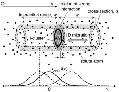
We proposed an analytical model for the total interaction energy between an interstitial cluster and solute atoms in binary alloys, as shown schematically in Figure 1. Strong interaction is expected for the solute atoms in a central core of the loop
dislocation. Letting the cross section of the annular region be
!
" (expressed by the number of atoms contained in the region), and letting the thickness be
!
b (i.e. the
atomic distance), then the volume of the region is
!
" atoms. The cross section
!
" will be in proportion to the length of the loop dislocation. The number of solute atoms
!
n(x)
in the region fluctuates with position
!
x of the cluster that glides along the direction of the Burgers vector. We consider also the weak interaction with solute atoms near the annular region by assuming an interaction potential upeak f (v) , where upeak is the peak
interaction energy and
!
f (v) is a non-dimensional function of the distance
!
v between the solute atom and the annular region in the
!
x direction. The function is
!
f (0) = 1, which decreases monotonically with increasing distance
!
v, and which is effectively
!
f (v) = 0 for
!
" > w ; the interaction range
!
w will be approximately 10b . The positive and negative values for upeak respectively represent repulsive and attractive
interactions.
For simplicity, we assume an identical interaction potential upeakf (v) for all
solute atoms the projection of which along
!
x direction are on the annular region, and ignore the other solute atoms. The total interaction energy in a solid solution is assumed to be given by a simple superposition of interaction potentials for individual solute atom, thereby by a convolution integral of the two functions as
u(x) = upeak f (v)n(x ! v) !w
w
"
dv . (1)Characteristics of the fluctuation in the total interaction energy u(x) are examined in
the following sections.
2.2. Outlines of the total interaction energy
The three functions presented above are considered at discrete points with an interval
!
b in the respective finite periods of nj = n jb
( )
and uj = u jb( )
forj = 0,1,!, L "1; fj = f jb
( )
for j = " L 2,!, "1, 0,1,!, L 2 "1. Parameter L , an evenas uj = upeak fq nj!q q=!L 2 L 2!1
"
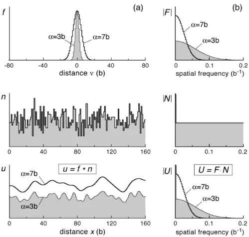
. (1’)Figure 2(a) portrays outlines of the three functions in a random alloy for solute concentration cs.
(1) The interaction potential is approximated as a Gaussian function
f (! ) = exp !!
(
2 "2)
, (2)where
!
" (> 0) is a constant representing the interaction range. The interaction energy decreases to upeake
!1
at ! = ±" . The figure shows cases for ! = 3b and ! = 7b .
(2) The number of solute atoms
!
nj in the annular region fluctuates with the migration distance of the interstitial cluster. Statistically,
!
nj follows the binomial
distribution Pb(n,!, cs) =! Cncs n
1! cs
(
)
! !n, which has average and variance asshown below:
E[n] = ! cs, V[n] = ! cs
(
1! cs)
. (3)(3) The total interaction energy
!
uj, a superposition of interaction potentials, shows periodic fluctuation with local peaks, i.e., smooth hills and valleys. The relation between
!
nj and uj is understood from the perspective that the convolution
operation in Eq. (1’) is a ‘moving average’ of
! nj using ! fj as weights. Because weight !
fj is a smoothing function, the averaging filters out fine scale fluctuations in
!
nj, and the trend remains in
!
uj. Larger ! averages over a longer range and results in smoother profiles.
2.3. Fourier spectrum of the total interaction energy
The three functions are described using Fourier analysis. Let Fk, Nk, and Uk
!
nj, and
!
uj. In the present convention, the discrete Fourier transform is, for example,
Uk = 1 L j=0uj L!1
"
e!i 2! Lkj k = 0,1,!, L !1. (4)It denotes the complex amplitude of the wave having wavelength
!
"= bL k. Also,
!
i is
an imaginary unit. Figure 2(b) presents outlines of the amplitude spectra in half of the frequency space because Fourier coefficients of real-valued functions are symmetrical at
!
k = 0.
(1) The Fourier transform of the function
!
fj for the interaction potential is another Gaussian function of real value, as
Fk=! 1 2" bL exp ! !2"2 b2L2 k 2 " # $ % & ' k = 0,1,!, L !1 . (5)
The spectrum involves a monotonic decrease at higher spatial frequencies. (2) The number of solute atoms
!
nj shows random fluctuation. Therefore, its Fourier transform has uniform intensity for all spatial frequencies except for
!
k = 0. It is
analogous to that of white noise as a function of time. The uniform power spectrum is expressed using the solute concentration cs and the interaction cross-section
!
"
(see Appendix A for the derivation), as
Nk2 =V[n]
L !1=
! cs(1! cs)
L !1 k = 1, 2,!, L !1. (6)
(3) A convolution operation in the spatial domain is expressed as a product in the frequency domain. Eq. (1’) is written as
Uk = upeakL Fk Nk. (7)
From Eqs. (5), (6), and (7), we obtain the intensity of the Fourier transform as
Uk2 =! cs(1! cs) L !1 " upeak 2 #2 b2 exp ! 2"2#2 b2L2 k 2 " # $ % & ' k = 1, 2,!, L !1. (8)
spectrum that is related to the wavelength of the smooth fluctuation in
!
uj. Therein,
Uk and Fk have an identical frequency dependence because of the uniform spectrum in Nk . In this sense, the characteristics of the fluctuation in
!
uj are analogous to those of white noise processed with a low-pass filter. In contrast, the pre-exponential factor in Eq. (8), which represents the overall intensity level of the spectrum, is directly proportional to the square of the average amplitude of the fluctuation in ! uj, as V[u] = Uk 2 k=1 L!1
"
#! cs(1! cs) L !1 " upeak 2 #2 b2 bL 2"#!1 $ % & ' ( ) # " 2 ! cs(1! cs)upeak 2 # b . (9)2.4. Variation of the total interaction energy
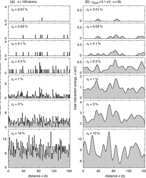
Figure 3 presents typical variation of
!
nj and
!
uj with the solute concentration
cs. In dilute alloys for ! cs<< 1 , the annular region contains no solute atom or
occasionally a single solute atom with probabilities P(0) = 1!! cs and P(1) = ! cs,
respectively [11]. The total interaction energy
!
uj has isolated peaks corresponding to solute atoms in the annular region. The height of peaks is upeak, and the mutual distance
xb obeys the geometrical distribution Pg(x,! cs) = ! cs
(
1!! cs)
x!1, as described in a previous report [11].
As the solute concentration increases to cs ! 1 2!"
(
)
, respective peaks mutually overlap. Further overlapping at higher cs does not flatten the energy profile but increases the fluctuation amplitude. Eq. (9) shows that V[u]1 2 is in proportion tocs 1 2 1! cs
(
)
1 2; note cs 1 2 1! cs(
)
1 2" cs 1 2for cs much lower than 50 atomic percent. The average amplitude of the fluctuation V[u]1 2 is also proportional to the peak interaction energy upeak, and to the square root of the interaction cross section !1 2
. We note that the relation reflects a fluctuation in the total number of solute atoms interacting with the loop dislocation. On the other hand, Eq. (8) shows that the wavelength of the fluctuation is independent of cs or !, but only on parameter ! for the interaction range.
Therefore, as a statistical average, uj varies only in the scale of the vertical axis in
proportion to cs 1 2
1! cs
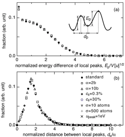
Figures 4(a) and 4(b) show distributions of the energy difference Ep and the
distance dp between the neighboring local peaks (i.e., hills and valleys) in the total
interaction energy
!
uj. Distance dp has a unique distribution when it is normalized by
the interaction range
!
" . Again it does not depend on cs or ! . The energy difference Ep has another unique distribution when it is normalized by V[u]
1 2
.
3. Atomistic simulations for the model 3.1. Description of the calculation cell
We conducted atomistic simulations of the interaction energy based on the MS method to examine the applicability of the analytical model proposed in Sec. 2. We selected Fe-Cu system with an interatomic potential given by Ackland et al. [24] that has been used for simulations of 1D migration [11,25,26]. The volume size factor of the solute copper atom in the iron lattice is about +8.8% in this potential function [24]. We induced solute copper atoms at random at concentrations up to 70 atomic percent to compare the results with the proposed model under various conditions. Although a random alloy is unrealistic at high solute concentrations because of low solubility of copper in iron, this study regards the system as an example of binary alloys. Hamaoka et al. conducted the HVEM experiments of 1D migration in Fe-Cu alloys from 0.005 to 0.9 at.%Cu [15].
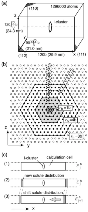
The calculation cell contained about 1.3 × 10⁶
mobile atoms, as shown in Figure 5(a). A periodic boundary condition was applied for all faces of the calculation cell at zero pressure. An interstitial cluster of a hexagonal plate was introduced at the cell center. The maximum radius rc of the interstitial cluster was 1b (7i), 4b (61i), or 8b (217i), as shown in Figure 5(b). Atoms on a hexagonal shell were grouped and labeled by the maximum radius rh of the shell. For example, all atoms on the edge of the
interstitial cluster 217i belong to a shell for rh = 8b .
3.2. Interaction between an interstitial cluster and a single solute copper atom
An interstitial cluster was fully relaxed in the iron lattice using the MS method. Then an iron atom in the cell was replaced by a copper atom. The interaction energy was estimated from the change in the total formation energy of the cell after relaxation. The typical error in estimating the formation energy was not larger than 0.005 eV. Each
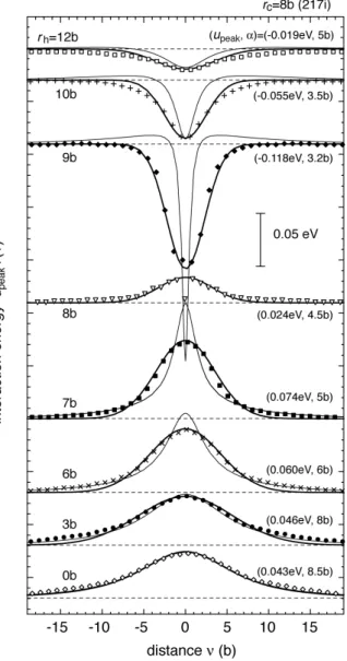
symbol in Figure 6(a) designates the interaction energy between an interstitial cluster (217i) and a solute atom in individual atomic row that is shown with broken circles in Figure 5(b), which corresponds to upeak fi in the model presented in Sec. 2. Bold lines
in Figure 6(a) are Gaussian functions fitted to the calculated results, with adoption of appropriate values for peak energy upeak and parameter
!
" for the interaction range. The interaction is repulsive for the solute atom in the atomic rows inside the loop
dislocation (rh< 8b ) because of the compressional strain, and is attractive on the outside
(rh> 8b ). The interaction is slight on the edge of the cluster ( rh= 8b ). Results for 7i
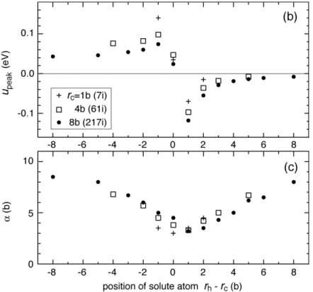
were described in earlier reports [11,26]. Figures 6(b) and 6(c) summarize the
parameters upeak and ! for the three cluster radii. They have similar variation to that
shown against rh! rc, the radial distance from the dislocation core. The difference in upeak was less than 0.022 eV for atomic rows between edge and corner positions (shown
with broken circles and a box, respectively in Figure 5(b)) within a hexagonal shell from rh= 6b to 12b in 217i. These results suggest that the long-range interaction
between the cluster and a solute atom is described better by defining the interaction potential for an individual shell.
3.3. Interaction energy in random Fe-Cu alloys
We calculated the total interaction energy corresponding to
!
uj in Sec. 2 according to the MS method shown schematically in Figure 5(c):
(1) The initial formation energy of the calculation cell is denoted as Eja
. (2) The solute atoms in the single atomic layer at the cell surface,
!
0 " x < b (shaded region in Figure 5(c)), were replaced by those with a new random distribution. The formation energy of the cell after relaxation was Ejb
. The difference Ejb ! Ej
a
resulted from the change in the number and the distribution of solute atoms in the surface layer. The interstitial cluster was far from the layer. Therefore, this
treatment was assumed not to affect the interaction energy between the cluster and solute atoms.
(3) The distribution of all the solute atoms in the cell was translated toward
!
"x
direction for a distance
!
b. This operation was done by switching the parameters
indicating atomic species without changing the atom coordinates. The formation energy of the cell after relaxation was Eaj+1. The difference Ej+1a ! Ej
b
was
a distance ! b toward ! + x direction, uj+1! uj= Ej+1 a ! Ej b .
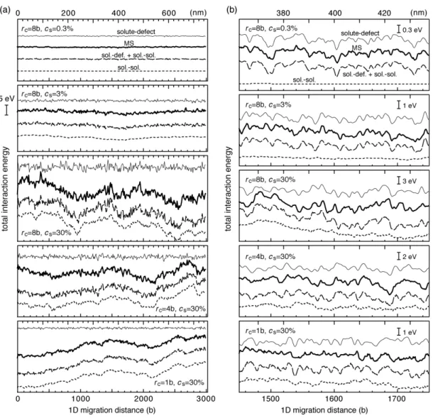
An iteration of the sequence produced a total interaction energy profile longer than the size of the calculation cell (i.e. 120 b) while introducing random solute distributions. Bold lines in Figure 7 show typical profiles of the interaction energy. The amplitude of the fluctuation in the interaction energy exceeded a few electron volts in concentrated alloys, even though the energy of the individual interaction potential was around 0.1 eV. The fluctuation will act as barriers for 1D migration of interstitial clusters larger than a few nano-meters.
3.4. Comparison between MS simulation and the analytical model
Thin lines in Figure 7 show the interaction energy in which interaction potentials
urh, peak frh, j were superposed according to the solute distribution nrh, j used in the MS calculation as uj = urh, peak frh, j nrh, j!q q=!L 2 L 2!1
"
rh"
. (1”)Suffix rh implies that the functions are defined for an individual hexagonal shell with radius
!
rh. The interaction potential urh, peak frh, j was produced with interpolation of
parameters urh, peak and !rh shown in Figures 6(b) and 6(c). The superposition
reproduces the MS results at low cs, but only the position and shape of individual local peak at high cs. Comparison of the two profiles at low magnification (Fig. 7(a)) reveals that the discrepancy at high cs results from slow fluctuation involved in the results of MS calculation. We describe in Sec. 4A that slow fluctuation arose from interaction among solute atoms (shown by dotted lines in Figure 7). We show in the following that the amplitude and wavelength of the fluctuation in
!
uj are fundamentally consistent with the analytical model.
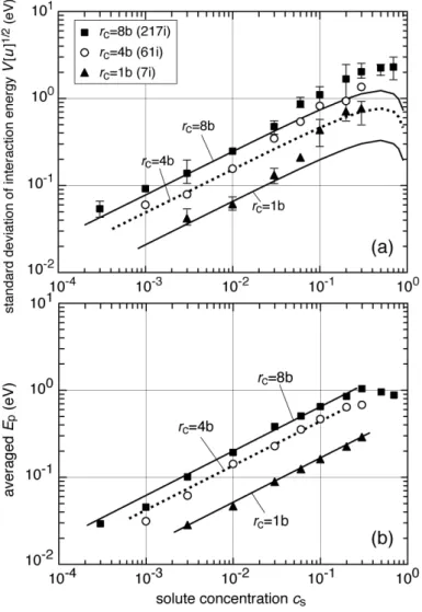
The symbols and lines presented in Figure 8(a) show a comparison of the average amplitude of the fluctuation V[u]1 2 between the MS calculation and the superposed interaction potentials. The latter was given by a sum of the variances for an individual shell as
V[u] ! ! 2 cs(1" cs) b "rh#rhurh, peak 2 2 rh
#
, (9’)because the contribution of the individual shell to the total variance was mutually independent. The average amplitude of the fluctuation V[u]1 2 for multiple shells is directly proportional to cs
1 2
1! cs
(
)
1 2. The two results show good correspondence at cslower than several atomic percent.
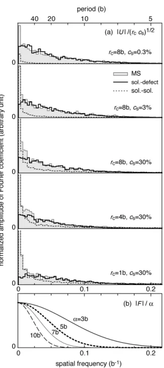
Shaded bars and bold lines in Figure 9(a) respectively show Fourier spectra Uk of the total interaction energy obtained using the MS calculation and the superposition. The two spectra show good correspondence at high frequencies. The discrepancy observed at very low frequencies is again caused by the contribution of the slow
fluctuation of the solute–solute interaction, as shown by dotted lines in Figure 9(a). The spectra for the superposition have similar frequency dependence, which are probably reproduced by an appropriate blending of the spectra for Gaussian functions from
!= 3b to 10b shown in Figure 9(b).
The energy difference Ep and distance dp of the neighboring peaks were
measured in the total interaction energy
!
uj obtained using the MS calculation. Figure 10(a) presents broad distributions of the energy difference Ep, whereas Figure 8(b)
shows that the average Ep is almost proportional to rc 1 2
and cs1 2. Effects of the slow fluctuation caused by solute–solute interaction were less apparent on the average Ep
than on V[u]1 2 shown in Figure 8(a). Figure 10(b) shows that dp is 0.5–2 nm, and
that its distribution apparently does not depend on cs or rc. These results are fundamentally consistent with the simple model, except for the difference in the distribution of dp. The fraction at short dp is larger for the MS results (Fig. 10(b))
than the simple model (Fig. 4(b)). The difference might be attributed to the interference of Gaussian functions among different upeak and ! in the MS calculation. Finally, we
note a correlation between the energy difference Ep and the distance dp; local peaks
with longer dp tend to have larger Ep, as shown in Figure 10(b). The correlation is
understood from the Fourier spectra: the lower amplitude at higher frequency allows only a smooth fluctuation in the spatial domain.
4. Discussion
4.1. Solute–solute interaction
Solute–solute interaction was ignored in the model described above. The interaction energy between two solute atoms was estimated from changes in the total formation energy of the calculation cell containing two solute atoms at various distances. The energy was -0.075 eV [24], -0.035 eV [24], and +0.020 eV, respectively, for pairs of the first-, second-, and third-nearest distances in the iron lattice; it was negligible for more distant pairs. The negative values denote attractive interactions. In this section, fluctuation in the solute–solute interaction energy of migrating interstitial clusters was examined to elucidate the characteristics of fluctuation in the total interaction energy, especially at higher cs.
1D migration of an interstitial cluster is regarded as a glide of the loop dislocation on the cylindrical glide plane. Simultaneously, the two parts of the crystal, i.e., inside and outside the glide cylinder, shift from each other by distance
!
b along the Burgers
vector. Figure 11(a) portrays configurational changes of close solute pairs as the
interstitial cluster migrates leftward. It is noteworthy that the figure shows an interstitial cluster fixed and solute atoms relative to the cluster. The changes in the mutual distance of solute pairs will change the interaction energy. We estimated the fluctuation in the total energy of solute–solute interaction based on the following assumptions: 1) we considered only the solute pairs for which the ‘atomic bond’ lies across the glide plane as shown in the top row in Figure 11(a). 2) We ignored gradual variation in the bond distance as the dislocation core passed by the solute pair. Instead we identified the first-, second-, and third-nearest pairs in the two states without the distortion that is apparent long before and after the passage of the dislocation core. We assumed that the two states were exchanged stepwise at the closest approach of the dislocation core. The solute pairs shown in the top row in Figure 11(a) are to change from (i) to (iii) stepwise at the dislocation core (ii). Then the number of close solute pairs in the calculation cell fluctuates with every 1D migration for distance
!
b. The fluctuation is a random walk
process, as described quantitatively in Appendix B.
From the fluctuation in the number of close solute pairs of the first-, second-, and third-nearest distances and the respective interaction energies, we estimated the
Figure 7. The number of close solute pairs is in direct proportion to cs2. Therefore, the fluctuation is negligible at low cs. The sum of solute–defect interaction and
solute–solute interaction is shown by broken lines, and better reproduces the MS results (bold lines) at high cs. Consequently, the characteristics of the fluctuation in the Fe-Cu system are described using a filtered white noise for solute–defect interaction and random walk for solute–solute interaction. The total energy of solute–solute interaction fluctuates more slowly than that of solute–defect interactions. This slow fluctuation is also apparent in the Fourier spectra portrayed in Figure 9(a). The solute–defect interaction (bold lines) had larger amplitude than the solute–solute interaction (dotted lines) at high spatial frequencies. The range of 1D migration is limited by the fast fluctuation in the solute–defect interaction. The wavelength of the fluctuation will be the characteristic length of 1D migration in concentrated alloys.
4.2. Solute–defect interaction
Interaction between a cluster and a single solute atom is the important element in the proposed model. In the classical theory of elasticity, the interaction energy between an inclusion at the cylindrical coordinate (r, z) and a circular dislocation loop of radius
R at the origin is given as [27]
E =!V 3"µ 1+# 1!# b R + r
(
)
2+ z2 R2 ! r2! z2 R ! r(
)
2+ z2E 4rR R + r(
)
2+ z2 " # $ $ % & ' '+ K 4rR R + r(
)
2+ z2 " # $ $ % & ' ' ( ) * * + , --, (10)where functions K(k) and E(k) are the complete elliptic integrals of the first and second kind. In addition, µ and ! respectively represent the shear modulus and Poisson’s ratio. Only the size misfit !V is the variable parameter. The peak interaction
energy depends on the misfit, but the interaction range does not. Thin lines in Figure 6(a) are interaction potentials for a solute atom with volume size factor of +15% in the iron lattice, which was chosen to correspond to the MS results in the atomic rows apart from the dislocation core, rh = 0b and rh= 12b . Near the dislocation core, however,
Eq. (10) gives interaction potentials with larger peak energy and smaller width. The singularities in the interaction energy at the dislocation core can be removed by introducing a constant A [28] into an expression for stress components of a circular dislocation loop [29]. Figure 12 (a) shows a variation of the interaction energy profiles
with the constant A for the atomic rows near the dislocation core. Profiles for A = 0
are identical to those of Eq. (10) [27] that were shown by thin lines in Figure 6(a). The divergent behavior in the profile is suppressed with increasing A . It is reported that
A ! 0.1R produces suitable interaction energy profile for very small interstitial clusters
(10i) [28]. For the present cluster (217i), profiles from A = 0.05R to A = 0.2R have the peak energy comparable to that of the MS results, but still have smaller peak width. We note that the elastic theory is better only for long-range interaction (i.e., !! 7b) inside the cluster rh = 7b ; the Gaussian functions decay too fast for the long-range. The same observation applies to rh = 6b and rh = 3b in Figure 6 (a). Because the
short-range interaction with larger energies has a large contribution to the total
interaction energy, the Gaussian function will be a better approximation for the present case.
Symbols in Figure 12 (b) show interatomic distance along the Burgers vector in the atomic rows examined in Figures 6(a). Thin lines are those derived from the
analytical solutions of the multistring Frenkel-Kontorova model for an edge dislocation and an interstitial cluster [30,31]: the atomic displacement of n -th atom in a string is given by un= b 2
(
)
! b(
!)
arctan n ! n(
(
0)
N)
, where n0 is the index of the centeratom of the crowdion. By adopting appropriate values for the parameter N, i.e., an effective dimensionless width of a crowdion, the solutions represent well the
interatomic distance un+1! un+ b of the atomic rows inside the cluster. A comparison
between Figures 6(a) and 12(b) suggests a rough relation between the displacement field and the interaction energy. Results for 7i are available in earlier report [11]. However, precise interaction energy profiles would not be obtained from the
displacement field. For example, the large displacement field observed in rh = 8b does not result in significant interaction energy. This might be explained partly by
displacement of the copper atom along the direction perpendicular to the Burgers vector; the oversized solute atom on the periphery of the interstitial cluster was found to displace outward for the distance around 0.01b.
Density functional calculations suggest an importance of chemical interactions in addition to solute size factor for the interaction between a single interstitial atom in iron and a solute atom, depending on the solute elements [32]. For the interaction with an interstitial cluster, however, few reports describe atomistic simulations using
semi-empirical interatomic potentials. In a Ni-Au system, gold is an oversized solute atom in nickel with an extremely large volume size factor: 63.6%. The activation energy for an interstitial cluster (7i and 19i) to overcome a gold atom inside the cluster is 0.8–1.0 eV [33], which will correspond to upeak in the system. Interaction in a Fe-Cr
system is reported using an advanced semi-empirical potential that is parameterized by application of the density functional theory [34]. The sign of the interaction is opposite that of Fe-Cu system. The solute chromium atom inside a cluster (7i, 37i, or 91i) has attractive interaction, and the peak energy upeak is from -0.1 to -0.2 eV for the solute
atom on the edge of the cluster. We estimated that the interaction potential corresponds to != 4b .
4.3. Fluctuation in interaction energy in alloys
Cottrell et al. [23] analyzed the fluctuation in the total interaction energy of interstitial clusters in alloys with application of the theory of solid solution hardening [35]. In solution hardening, a flexible dislocation line of infinite length gains potential energy by adjusting its shape along valleys in a field of randomly arranged energy hills and valleys, where the dislocation must bow out at least the distance
!
w, the range of interaction between dislocation and a solute atom. A critical length of dislocation segment, called the Labusch length, exists as
!L = Tw 2 ˆU cs 1 2 ! " # $ % & 2 3 , (11)
where T is the line tension and ˆU corresponds to upeak in our notation. The
fluctuation of potential energy on the scale !L has amplitude of EL = T 2 ! " # $ % & 1 3 w4 3 ˆ U2 3 cs 1 3 . (12)
Dislocations can bow out only in scales larger than !L because bowing out in smaller
scales involves an increase in the line energy in excess of the gain in the potential energy. Such a dislocation is pinned by the fluctuation of the solute distribution, in the sense that the interaction energy must increase to pass over a hill-top into the next valley. The dislocation needs an external energy supply to move. In the solution
hardening the pinning energy is equivalent to the net energy gain. Cottrell et al.
proposed the pinning energy for a dislocation loop of finite perimeter length nb under no driving stress acting on the loop [23],
E ! EL nb !L " # $ % & ' 1 3 . (13)
The pinning energy for 217i was estimated as 0.003, 0.09, and 0.26 eV for Fe-0.3%, 3%, and 30% Cu, respectively, with adoption of ˆU = 0.1 eV , nb = 50 b ,
w =1 b , and Tb =1 eV in Eqs. (11)–(13). The latter two parameters were after Cottrell
et al. for iron-based alloys [23]. The pinning energies were much lower than the average
Ep in the MS results presented in Figure 8(b). Parameter w =1 b represents a
short-range interaction for solute atoms in the central core of the loop dislocation, ignoring the contribution of longer-range interaction. However, Figure 3 demonstrated a considerable difference in the interaction energy profiles between the short-range
interaction upeak nj and the long-range interaction uj. When we adopted w = 5 b , the
pinning energy increased to 0.20, 0.55, and 1.54 eV, respectively, which were
comparable to the average Ep. We still note substantial differences between Cottrell’s
model and the MS results on Fe-Cu alloys: 1) We did not observe the loop dislocation to
bow out in deflection as long as w = 5 b during MD or MS simulations when we
visualized the central core of the loop dislocation using the Wigner–Seitz cell method. 2) The typical pinning energy was directly proportional to cs
4 9r c
1 3
in Cottrell’s model but to cs1 2rc1 2
for Fe-Cu alloys. The total interaction energy was interpreted better by the superposition of cluster–solute interaction and solute–solute interaction, neither of which considered the energy gain by bowing out of the loop dislocation.
4.4. Brief comments
Fluctuation in the total interaction energy is expected to affect dynamic processes of 1D migration in alloys, depending on the temperature, species, concentrations of solute elements, and cluster size. Intermittent 1D migration is observed for interstitial clusters of a few nanometers in diameter under electron irradiation [9,10,13-15]. The 1D migration distance has a common distribution among the alloys examined. The fraction decreases concomitantly with increasing 1D migration distance, and the distance only slightly exceeds 10 nm. There would be a common mechanism for the distribution of
1D migration distance in these concentrated alloys. Our tentative model of experimental 1D migration is in the following. Interstitial clusters are in a stationary state in
concentrated alloys, at a position where the formation energy of the clusters achieves a local minimum on their respective 1D migration tracks. The distribution of solute atoms is expected to change continuously from one random distribution to another (both are equivalent to each other) under electron irradiation because of displacement of atoms and the following recovery of produced Frenkel pairs. This ‘mixing’ effect of solute atoms changes the stable position of the cluster on its 1D migration track, and the clusters induce 1D migration into a new stable position. We presume that the experimental 1D migration distance reflects the wavelength of the fluctuation in the total interaction energy.
Atomistic simulations of diffusion coefficients of 1D migration have been reported for Fe-Cu and Fe-Cr alloys [25,36]. It is reported that the solute concentration dependence of 1D migration diffusivity (7i-91i) is not monotonous in Fe-Cr alloys; the diffusivity has a lower peak around 10 at.% Cr [36]. We have conducted dynamic simulations of 1D migration in Fe-Cu alloys in which we examined the behavior of interstitial clusters in terms of the fluctuation in the interaction energy. We also examined the mechanism of initiation of 1D migration under electron irradiation to elucidate the experimental 1D migration behavior in alloys. Those results will be presented elsewhere.
5. Conclusion
For understanding and modeling of 1D migration of interstitial clusters in dilute and concentrated alloys, we studied characteristics of the fluctuation in the formation energy of interstitial clusters gliding along the Burgers vector. We proposed and examined two mechanisms of the fluctuation, which were solute–defect and solute–solute interactions, each of which reflects fluctuation in the microscopic distribution of solute atoms in terms of the cluster.
For the solute–defect interaction, the total interaction energy was assumed to be a superposition of a Gaussian function representing long-range interaction between the cluster and individual solute atom. An application of the model to random binary alloys revealed that the characteristics of the fluctuation resembled those of white noise processed with a low-pass filter. The average energy difference of the neighboring local
peaks in the fluctuation was directly proportional to the square root of both the solute concentration cs and the cluster radius rc. The distribution of the distance separating local peaks was virtually independent of cs and rc, but was dependent only on the range of the interaction potential. For the solute–solute interaction, we considered the fluctuation in the number of close solute pairs caused by the mutual shift of the crystal inside and outside of the cylindrical glide plane. The fluctuation was a kind of random walk process, and was effective for cs higher than a few percent.
The models interpreted the results of MS simulation for fluctuating interaction energy in Fe-Cu alloys under systematically varied conditions. The typical energy height of local peaks exceeded a few electron volts in concentrated alloys, even though the energy of individual solute–defect interaction was around 0.1 eV. The distance between local peaks ranged up to 2 nm. The wavelength of the fluctuation attributable to the solute–defect interaction would be the characteristic length of 1D migration in concentrated alloys. The wavelength was thought to be responsible for the short-range 1D migration of interstitial clusters observed in various alloys under electron irradiation.
Acknowledgements
This work was supported by a Grant-in-Aid for Scientific Research from the Ministry of Education, Science, and Culture of Japan (No. 21560868). A part of the numerical simulation was performed using the Center for Computational Materials Science, Institute for Materials Research, Tohoku University (Proposal No. 12S0408).
References
[1] A.I.J. Foreman, W.J. Phythian, and C.A. English, Philos. Mag. A 66, 671-695 (1992).
[2] A.F. Calder and D.J. Bacon, J. Nucl. Mater. 207, 25-45 (1993).
[3] W.J. Phythian, R.E. Stoller, A.E.J. Foreman, A.E. Calder, and D.J. Bacon, J. Nucl. Mater. 223, 245-261 (1995).
[4] B.D. Wirth, G.R. Odette, D. Maroudas, and G.E. Lucas, J. Nucl. Mater. 244, 185-194 (1997).
[5] N. Soneda and T. Diaz de la Rubia, Philos. Mag. 81, 331-343 (2001).
[6] Yu.N. Osetskey, D.J. Bacon, A. Serra, B.N. Singh, and S.I. Golubov, Philos. Mag.
[7] E. Kuramoto, J. Nucl. Mater. 276 (2000) 143-153. [8] M. Kiritani, J. Nucl. Mater. 251, 237-251 (1997).
[9] T. Hayashi, K. Fukumoto, and H. Matsui, J. Nucl. Mater. 307-311, 993-997 (2002). [10] K. Arakawa, M. Hatanaka, H. Mori, and K.Ono, J. Nucl. Mater. 329-333,
1194-1198 (2004).
[11] Y. Satoh, H. Matsui, and T. Hamaoka, Phys. Rev. B 77, 094135 (2008). [12] Y. Satoh and H. Matsui, Philos. Mag. 89, 1489-1504 (2009).
[13] T. Hamaoka, Y. Satoh, and H. Matsui, J. Nucl. Mater. 399, 26-31 (2010). [14] Y. Satoh, H. Abe, and S.W. Kim, Philos. Mag. 92, 1129-1148 (2012). [15] T. Hamaoka, Y. Satoh, and H. Matsui, J. Nucl. Mater. in press.
[16] D.A. Terentyev, L. Malerba, and M. Hou, Phys. Rev. B 75, 104108 (2007). [17] M. Pelfort, Yu.N. Osetsky, and A. Serra, Philos. Mag. Lett. 81, 803-811 (2001). [18] S.L. Dudarev, M.R. Gilbert, K. Arakawa, H. Mori, Z. Yao, M.L. Jenkins, and P.M. Derlet, Phys. Rev. B 81, 224107 (2010).
[19] K. Arakawa, K.Ono, M. Isshiki, K. Mimura, M. Uchikoshi, and H. Mori, Science
318, 956-959 (2007).
[20] D. Terentyev, N. Anento, A. Serra, V. Jansson, H. Khater, and G. Bonny, J. Nucl. Mater. 408, 272-284 (2011).
[21] D.A. Terentyev, T.P.C. Klaver, P. Olsson, M.-C. Marinica, F. Williame, C. Domain, and L. Malerba, Phys. Rev. Lett. 100, 145503 (2008).
[22] S.L. Dudarev, P.M. Derlet, and C.H. Woo, Nucl. Inst. Meth. Phys. Res. B 256, 253-259 (2007).
[23] G.A. Cottrell, S.L. Dudarev, and R.A. Forrest, J. Nucl. Mater. 325, 195-201 (2004). [24] G.J. Ackland, D.J. Bacon, and A.F. Calder, T. Harry, Philos. Mag. 75, 713-732 (1997).
[25] J. Marian, B.D. Wirth, A. Caro, B. Sadigh, G.R. Odette, J.M. Perlado, and T. Diaz de la Rubia, Phys. Rev. B 65, 144102 (2002).
[26] A.C. Arokiam, A.V. Barashev, D.J. Bacon, and Y.N. Osetsky, Philos. Mag. 87, 925-943 (2007).
[27] J. Bastecka and F. Kroupa, Czech. J. Phys. B 14, 443-453 (1964).
[28] T.S. Hudson, S.L. Dudarev, and A.P. Sutton, Proc.R. Soc. Lond. A 460, 2457-2475 (2004).
81, 583-593 (2001).
[30] S.L. Dudarev, Philos. Mag. 83, 3577-3597 (2003).
[31] D. Nguyen-Manh, A.P.Horsfield, and S.L. Dudarev, Phys. Rev. B 73, 020101 (2006).
[32] P. Olsson, T.P.C. Klaver, and C. Domain, Phys. Rev. B 81, 054102 (2010). [33] K. Sato, T. Yoshiie, and Q. Xu, J. Nucl. Mater. 367-370, 382-385 (2007). [34] D. Terentyev, P. Olsson, L. Malerba, and A.V. Barashev, J. Nucl. Mater. 362, 167-173 (2007).
[35] M. Zaiser, Philos. Mag. 81, 2869-2883 (2002).
[36] D. Terentyev, L. Malerba, and A.V. Barashev, Philos. Mag. Lett. 85, 587-594 (2005).
Appendix A
This section presents derivation of the power spectrum of the number of solute atoms
!
nj in the central core of a cluster. Parseval’s theorem shows that the Fourier transform preserves the energy of the original quantity. For real-valued function
! nj, ! 1 L nj 2 j= 0 L"1
#
= Nk2 k= 0 L"1#
. (A1)The left term of Eq. (A1) represents E[n2]. Consequently, the average and the variance of the function
!
nj are related to the Fourier coefficients as
E[n] =1 L j=0nj L!1
"
= N0, V[n] = E[n2]! E[n]2 = Nk2 k=1 L!1"
. (A2)The power spectrum Nk
2
is uniform except for
!
k = 0 because of a random variation
in
!
nj. Then we obtain Eq. (6).
Appendix B
This section presents a description of a quantitative analysis of the fluctuation in the total number of close solute pairs as an interstitial cluster glide along the Burgers vector. In the model presented in Sec. 4A, the close atomic sites AB that lie across the glide plane are replaced by AC at the dislocation core, as shown in Figure 11 (a). Let the
number of such replacements around the cluster be m by every 1D migration for the
distance
!
b. For example, m for the first, second, and third nearest sites is estimated,
respectively, as 102, 102, and 252 around 217i, and 18, 18, and 42 for 7i.
We assume a random distribution of solute atoms at concentration cs. The
probability of finding x solute atoms on m sites A is given by the binomial
probability distribution Pb(x, m, cs) =x Cm cs x
1! cs
(
)
n!x. Similarly, the probability of finding y (! x) solute pairs on m sites AB is given as Pb(x, m, cs)Pb(y, x, cs)x=0 m
!
orPb(y, m, cs2) . A glide of the cluster for the distance
!
b induces m replacements from
AB to AC, and the number of close solute pairs will increase, decrease, or stay
unchanged depending on the solute distribution on sites A, B, and C. The probability of changing ! solute pairs is expressed as
P(±!) = Pb(x, m, cs) Pb(y, x, cs) y=0 m
"
Pb(y + !, x, cs) x=0 m"
. (B1)The typical probability distributions are shown in Figure 11(b). The probability takes the maximum at ! = 0, and is symmetrical at ! = 0. Probability P(!) can be
approximated by a normal distribution shown by thin lines for large clusters (with large
m ) at high cs.
In successive glide motions of a cluster in random alloys, changes ! in
individual steps will be mutually independent. Therefore, the fluctuation in the number of close solute pairs is a kind of random-walk processes. In the well-known ‘simple random walk’, a particle moves +1 or -1 with equal probability at each step. The normal distribution in ! suggests that the present fluctuation can be described better as
Figure 1. Schematic illustration of the present model describing the total interaction energy between an interstitial cluster and solute atoms in random binary alloys.
Figure 2. Typical profiles of the interaction potential
!
fj, the number of solute atoms
!
nj in the region of strong interaction, and total interaction energy
!
uj, in (a) the spatial domain and (b) the frequency domain (Fourier spectra). Symbol * denotes the
convolution operation. Parameter
!
Figure 3. Typical variation of (a) the number of solute atoms
!
nj in the region of strong interaction, and (b) the corresponding total interaction energy
!
uj with the solute concentration cs.
!
Figure 4. Normalized distributions of (a) the energy difference Ep and (b) the distance dp of the neighboring local peaks in the total interaction energy
!
uj. The standard condition was ! =5b, cs=3%,
!
"=100 atoms, and upeak=+0.1 eV. Only the indicated
Figure 5. (a) Geometry of the calculation cell used in the atomistic simulations based on the MS method. (b) Configuration of the interstitial cluster observed along the
!
x
direction. Full and open circles respectively correspond to atomic rows with and without the extra plane of 217i. Shaded hexagons show 61i and 7i. (c) Method of calculation of the total interaction energy between an interstitial cluster and solute atoms.
Figure 6. (a) Interaction energy between an interstitial cluster (217i) and a solute copper atom in atomic rows from rh= 0b to rh= 12b as a function of mutual distance
!
v in the
!
x direction (see Figure 1(a)). Symbols show the results of MS calculation. Bold
lines are the Gaussian function upeakexp !v 2
!2
(
)
fitted to the MS results. Interactionenergy below the broken lines represents attractive interaction. The solute atom was placed on the atomic rows shown by broken circles in Figure 5(b). Thin lines show the interaction energy between a circular loop and an inclusion according to the elastic theory: R = 8.5b and !V = 1.21Ao 3 in Eq. (10).
Figure 6. (b) (c) Variation of upeak and ! with radii of the interstitial cluster rc and
Figure 7. Fluctuation in the total interaction energy between an interstitial cluster and solute atoms in a random alloy as a function of the 1D migration distance of the cluster. Bold lines show results of MS calculations. Thin lines show the superposition of
interaction potentials given by Eq. (1”). Dotted lines show contributions of the solute–solute interaction. Results are shown at the common scale in (a), and are magnified for individual conditions in (b).
Figure 8. (a) Standard deviation of the total interaction energy as a function of the solute concentration cs and the radius rc of the interstitial cluster. Symbols and lines
respectively show results of MS calculation and superposition of interaction potentials.
L = 500b. (b) Averaged energy difference Ep of the neighboring peaks in the total interaction energy obtained by MS calculation as a function of cs and rc. Lines show
cs 1/2
Figure 9. (a) Normalized Fourier spectra of the total interaction energy profiles
compared among MS method, superposition of interaction potentials, and solute–solute interaction. The Hamming window function was applied before the Fourier transform to
reduce the boundary effect. L = 1200b. (b) Normalized Fourier spectra of Gaussian
Figure 10. Typical distributions of (a) the energy difference Ep and (b) the mutual
distance dp of the neighboring local peaks in the total interaction energy
!
uj
estimated using MS method. Symbols and error bars in (b) show the average, and the upper and lower quartiles of Ep for individual bins of the histogram.
Figure 11. (a) Schematic illustration of the model describing the changes in
solute–solute interaction by 1D migration of interstitial clusters in random binary alloys. (b) Typical probability distributions of the change ! in the number of close solute pairs by the 1D migration of interstitial cluster for distance
!
b. Thin lines show normal
Figure 12. (a) Interaction energy between an interstitial cluster (217i) and a solute copper atom in atomic rows from rh = 7b to rh= 9b as a function of mutual distance
!
v in the
!
x direction. Symbols and bold lines are the MS results and the Gaussian functions, which were already shown in Figure 6(a). Thin lines show the interaction energy according to the elastic theory [28,29]: R = 8.5b and !V = 1.21A
o 3
. (b)
Interatomic distance along the Burgers vector. Symbols and thick lines are the results of MS calculation for the atomic rows identical to those in Figure 6(a). Thin lines show analytical solutions of the multistring Frenkel-Kontorova model [30]; the parameter N representing the effective width of a crowdion was fitted to the MS results.