Monodromy of Painleve VI Equation Around Classical Special Solutions (Monodromy of the differential equations and related problems)

Monodromy

of

Painlev\’e

_VI

Equation

Around

Classical

Special

Solutions*

Katsunori

Iwasaki (

岩崎克則

)

Faculty

of

Mathematics,

Kyushu University

6-10-1

Hakozaki,

Higashi-ku, Fukuoka

812-8581

Japan

March

29,

2009

Abstract

A global structure ofthe sixthPainlev\’eequationis described by itsnonlinear

mon-odromy map along a loop, and it is interesting to investigate its dynamical properties around classical special solutions, that is, around Gauss $hyperg\infty metric$ function

solu-tions. In ageneric situationone

sees

that the monodromymap admitsahorseshoe and

thus exhibits achaotic behavior in any small neighborhood of the classical solutions.

1

Introduction

This is a report of a work [11] in progress conceming the monodromy ofthe sixth Painlev\’e

equation and the associated dynamical system created by a monodromy map.

In general, a total understanding of the Painlev\’e equation would be achieved by the

scheme in Table 1, in which

some

typical issues in various scales

are

listed, from microlocal

to macroscopic levels. Recent works by the author and his coworkers

are

mainly concerned

with global-txmacroscopic structures of the Painlev\’e equation. Usually,

some

properties of

this equationhavebeen studied from the viewpointof isomonodromic deformations, but this

approach is often too local in many respects. One should take

more

global points ofview.

A global structure of the Painlev\’e equation is represented by the nonlinear monodromy

map (of a single turn along

a

given loop). A clear picture of this part is made by

estab-lishing

a

very precise Riemann-Hilbert correspondence based

on a

suitable moduli theory in

algebraic geometry. An even more global (namely, macroscopic) structure of the equation

is represented by the iterations of the monodromy map, that is, by infinitely many turns of

the loop. Dynamical systems theory and ergodic theory

come

into context at this stage.

In the linear

case

of Gauss hypergeometric equation, the monodromy map of a single

turn and its iterations ofinfinitely many tums make no essential difference, since the former is only a linear map and the dominant effect of the latter is controlled by the spectral data

Table 1: A total understanding of Painlev\’e equation

of the former, namely, by the largest eigenvalue and its eigenspace. In the nonlinear

case

of

Painlev\’e equation, there exists

a

large gap between the single tum and the infinitely many

tums, dueto the ”nonlinear effect” ofPainlev\’e equation. The analysis of the latter requires

advanced methods from dynamical systems theory and ergodic theory. But this leads to the

new

feature of

a

chaotic dynamicalsystem, which

never

exists in Gauss equation and which

makes the global structure of Painlev\’e equation much

more

interesting than that of Gauss

equation. We

are

interested in such

an

aspect of Painlev\’e equation.

The main focus of this paper is

on a

chaotic nature ofPainlev\’e equation around classical specialsolutions, that is, around Gauss hypergeometricfunction solutions (orinotherwords,

Riccati solutions). The Riccati solutions

are

parametrized by a

curve

called the Riccati

curve.

In this paper

we announce

the following result: In any small neighborhood of the

Riccati

curve

the nonlinear monodromy map admits

a

Smale horseshoe and thus exhibits

a

very complicated dynamical behavior, for almost all loops and for almost all parameters for which Painlev\’e equation admits Riccati solutions. See Result 4 for the precise statement.

2

The

Sixth

Painlev\’e

Equation

The sixth Painlev\’e equation $P_{VI}(\kappa)$ is a Hamiltonian system

$\frac{dq}{dz}=\frac{\partial H(\kappa)}{\partial p}$, $\frac{dp}{dz}=-\frac{\partial H(\kappa)}{\partial q}$, (1)

with

a

complex time variable $z\in Z:=\mathbb{P}^{1}-\{0,1, \infty\}$ and unknown functions $q=q(z)$ and

$p=p(z)$, depending

on

complex parameters $\kappa$ in the four-dimensional affine space

$\mathcal{K}:=\{\kappa=(\kappa_{0}, \kappa_{1}, \kappa_{2_{1}}\kappa_{3}, \kappa_{4})\in \mathbb{C}_{\kappa}^{5}:2\kappa_{0}+\kappa_{1}+\kappa_{2}+\kappa_{3}+\kappa_{4}=1\}$ ,

where the Hamiltonian $H(\kappa)=H(q,p, z;\kappa)$ is given by

$z(z-1)H(\kappa)=(q_{0}q_{z}q_{1})p^{2}-\{\kappa_{1}q_{1}q_{z}+(\kappa_{2}-1)q_{0}q_{1}+\kappa_{3}q_{0}q_{z}\}p+\kappa_{0}(\kappa_{0}+\kappa_{4})q_{z}$,

with $q_{\nu}$ $:=q-\nu$ for $\nu\in\{0, z, 1\}$

.

Note that $P_{VI}(\kappa)$ fails to make

sense

at $z=0,1,$$\infty$

.

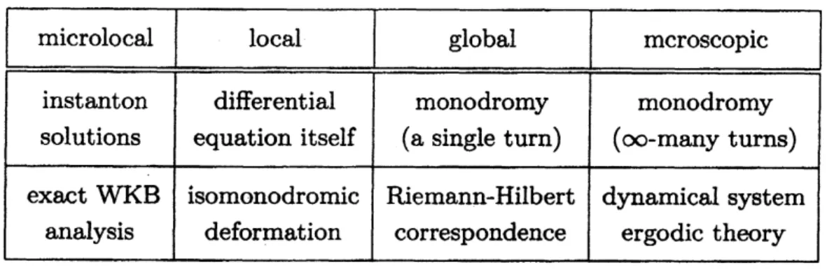
These

Figure 1: Monodromy map $\gamma_{*}:$ $\mathcal{M}_{z}(\kappa)O$ along

a

loop $\gamma\in\pi_{1}(Z, z)$

.

3

Moduli

Theory

Let $\mathcal{M}_{z}(\kappa)$ be the set of all meromorphic solution germs to $P_{VI}(\kappa)$ at

a

base point $z\in Z$

.

The set $\mathcal{M}_{z}(\kappa)$

can

be realized

as

the moduli space of (certain) stable parabolic connections,

so

that it

can

be equiped with the structure of a smooth quasi-projective rational complex

surface [6, 7, 8], where

a

stable parabolic connection is

a

rank-two vector bundle

over

$\mathbb{P}^{1}$

together with

a

FMchsian connection having four regular singular points and

a

parabolic

structure that satisfies a sort ofstability condition in geometric invariant theory.

Moreover there exists

a

natural compactification of the moduli space

$\mathcal{M}_{z}(\kappa)arrow\overline{\mathcal{M}}_{z}(\kappa)$,

where $\overline{\mathcal{M}}_{z}(\kappa)$ is the moduli space of stable parabolic phi-connections. Here, roughly

speak-ing, a stable parabolic phi-connection “V $=\phi\otimes d+A$” is a variant of stable parabolic

connection allowing a “matrix-valued Planck constant” $\phi$, called

a

phi-field (that may be

degenerate

or

semi-classical). The compactified modulis space $\overline{\mathcal{M}}_{z}(\kappa)$ has

a

unique

anti-canonical effective divisor $\mathcal{Y}_{z}(\kappa)$, which has the irreducible decomposition

$\mathcal{Y}_{z}(\kappa)=2E_{0}+E_{1}+E_{2}+E_{3}+E_{4}$

.

(2)

The objects

on

$\mathcal{Y}_{z}(\kappa)$

are

exactly those with degenerate phi-field $\phi$, where the coefficientsof

the irreducible decomposition (2) stand for the ranks ofdegeneracy of $\phi$

.

Thus one has

$\mathcal{M}_{z}(\kappa)=\overline{\mathcal{M}}_{z}(\kappa)-\mathcal{Y}_{z}(\kappa)$,

and there exists a holomorphic two-form $\omega_{z}(\kappa)$

on

$\mathcal{M}_{z}(\kappa)$, meromorphic

on

$\overline{\mathcal{M}}_{z}(\kappa)$ with

pole divisor $\mathcal{Y}_{z}(\kappa)$

.

It is unique up to constant multiples and yields

a

natural holomorphic area-form

on

the moduli space $\mathcal{M}_{z}(\kappa)$

.

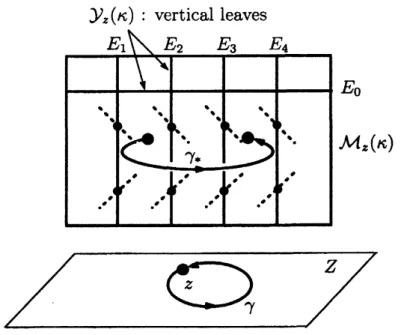
Figure 2: Three basic loops in $\pi_{1}(Z, z)$, where $z_{1}=0,$ $z_{2}=1$ and $z_{3}=\infty$

.

4

Nonlinear

Monodromy

It is known that $P_{VI}(\kappa)$ enjoys the Painlev\’eproperty, that is, any solution germ $Q\in \mathcal{M}_{z}(\kappa)$

can

be continued analytically alonganyloop$\gamma\in\pi_{1}(Z, z)$

as a

meromorphicfunction. Thanks

to this property, the monodromy map along the loop $\gamma$,

$\gamma_{*}:\mathcal{M}_{z}(\kappa)arrow \mathcal{M}_{z}(\kappa)$, $Q\mapsto\gamma_{*}Q$, (3)

$is$ well defined, where $\gamma_{*}Q$ is the result of the analytic continuation (see Figure 1). It is

a

holomorphic automorphism of $\mathcal{M}_{z}(\kappa)$ preserving the holomorphic area-form $\omega_{z}(\kappa)$

.

We are interested in the dynamics of the monodromy map $\gamma_{*}:\mathcal{M}_{z}(\kappa)CJ$ along a given

loop $\gamma\in\pi_{1}(Z, z)$

.

The fundamental group $\pi_{1}(Z, z)$ is represented

as

$\pi_{1}(Z, z)=\{\gamma_{1},$ $\gamma_{2},\gamma_{3}|\gamma_{1}\gamma_{2}\gamma_{3}=1\rangle$,

where $\gamma_{i}(i=1,2,3)$

are

the basic loops

as

in Figure 2, with $z_{1}=0,$ $z_{2}=1$ and $z_{3}=\infty$

.

Deflnition 1 A loop $\gamma\in\pi_{1}(Z, z)$ is said to be elementaryif $\gamma$ is conjugate to the loop $\gamma_{i}^{m}$

for

some

$i\in\{1,2,3\}$ and $m\in Z$, namely, if it makes a finite number of tums around only

one

of the three fixed singular points. Otherwise, $\gamma$ is said to be non-elementary.

The dynamics along an elementary loop is relatively simpler [10, 13] and

we are more

inter-ested in the dynamics along a non-elementary loop.

5

Riccati Curves

For particular parameters $\kappa$ of codimension

one

in $\mathcal{K}$, there exist particular solutions

to

$P_{VI}(\kappa)$ that

can

be expressed in terms of Gauss hypergeometric functions. They

are

known

as

Riccati solutions,

as

they appear

as

solutions to the Riccati equation associated with

a

Gaussequation. Let$\mathcal{E}_{z}(\kappa)$ be thesetof all Riccatisolution germsto $P_{VI}(\kappa)$ atthe basepoint $z$

.

It is known that $\mathcal{E}_{z}(\kappa)$ is

an

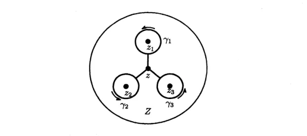
algebraic set in $\mathcal{M}_{z}(\kappa)$, each irreducible component of which

$1_{\bullet}$ $\bullet^{2}$ $\emptyset’0\cdot\cdot\cdot\cdot$

.

$’$ $a$

...

$3^{\bullet}$

.

$\bullet_{4}$ $A_{1}^{\oplus 4}$

$I=\{0,1,2,3\}$ $I=\{1,2,3,4\}$ $I=\{0,1,2\}$

Figure 3: Some strata and their abstract Dynkin types

number-2. Conversely, any (-2)-curve in $\mathcal{M}_{z}(\kappa)$ is

an

irreducible component of$\mathcal{E}_{z}(\kappa)$

.

For

this

reason a

(-2)-curve is called a Riccati

curve.

We

can

think of the dual graph of $\mathcal{E}_{z}(\kappa)$

which encodes the intersection relations among the Riccati

curves

in $\mathcal{M}_{z}(\kappa)$

.

6

Affine Weyl Groups

The configurationofRiccati

curves

in $\mathcal{M}_{z}(\kappa)$

can

most clearly be described in termsof

some

affine Weyl group structures and

an

associated stratification

on

$\mathcal{K}$ (see Lemma 2). Consider

the (complex) innerproduct

on

$\mathcal{K}$ induced from the standard Euclidean innerproduct

on

$\mathbb{C}_{\kappa}^{4}$

through the forgetful isomorphism $\mathcal{K}arrow \mathbb{C}_{\kappa}^{4},$ $\kappa\mapsto(\kappa_{1}, \kappa_{2}, \kappa_{3}, \kappa_{4})$

.

For each $i\in\{0,1,2,3,4\}$

let $w_{i}$

:

$\mathcal{K}0$ be the orthogonal reflection in the affine hyperplane $H_{i};=\{\kappa\in \mathcal{K} : \kappa_{i}=0\}$

.

These five reflections generate

an

affine Weyl

group

oftype $D_{4}^{(1)}$,

$W(D_{4}^{(1)})=\{w_{0}, w_{1}, w_{2}, w_{3}, w_{4}\}\cap \mathcal{K}$

.

Denote the nodes of the Dynkin diagram $D_{4}^{(1)}$ by _{$\{0,1,2,3,4\}$}, where $0$ represents the

central node. The automorphism group ofthe Dynkin diagram $D_{4}^{(1)}$ is the symmetric group $S_{4}$ of degree 4 permuting

{1,

2,3,

4}

while fixing the central node $0$

.

The semi-direct product

$W(F_{4}^{(1)}):=W(D_{4}^{(1)})xS_{4^{\Gamma}}\backslash \mathcal{K}$

is

an

affine Weyl group of type $F_{4}^{(1)}$, which is the full symmetry group of Painlev\’e VI.

7

Stratification

There exists

a

natural stratification of $\mathcal{K}$, namely, the

one

by proper subdiagrams of the

Dynkin diagram $D_{4}^{(1)}$, which

we

shall

now

describe. Let _{$\mathcal{I}:=\{I\subset\{0,1,2,3,4\}\}/S_{4}$} be the

set of all proper subsets of $\{0,1,2,3,4\}$, including the empty set $\emptyset$, up to the action of $S_{4}$

.

Note that each element of$\mathcal{I}$ represents the abstract Dynkin type ofa proper subdiagram of

$D_{4}^{(1)}$

.

For each _{$[I]\in \mathcal{I}$} with _{$I\subset\{0,1,2,3,4\}$}

we

put

$\overline{\mathcal{K}}([I])$ _$=$ the $W(F_{4}^{(1)})$-translates of the affine subspace $H_{I}$

$:= \bigcap_{i\in I}H_{i}$, $\mathcal{K}([I])$ $=$

Xlf

$([I])- \bigcup_{|J|=|t|+1}\overline{\mathcal{K}}([J])$, where

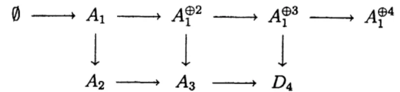
$\emptysetarrow A_{1}arrow A_{1}^{\oplus 2}arrow A_{1}^{\oplus 3}arrow A_{1}^{\oplus 4}$

$\downarrow$ $\downarrow$ $\downarrow$

$A_{2}arrow A_{3}$ $arrow D_{4}$

Figure 4: Adjacency relations among the strata

The sets $\mathcal{K}(*)$ with $*\in \mathcal{I}$define

a

stratification of$\mathcal{K}$

.

For$I=\emptyset$

one

has the big

open stratum

$\mathcal{K}(\emptyset)$ and

some

other strata

are

given in Figure 3.

The adjacency relationsamong the strata

are depicted in Figure 4, _where $*arrow**$ indicates that $\mathcal{K}(**)$ is in the closure of $\mathcal{K}(*)$

.

Lemma 2

_If

$\kappa\in \mathcal{K}(*)with*\in \mathcal{I}$, then the dual graph

of

$\mathcal{E}_{z}(\kappa)\subset \mathcal{M}_{z}(\kappa)$ is the Dynkin

graph

_of

$type*$

.

In particular$\mathcal{M}_{z}(\kappa)$ contains

no

Riccati

curve

precisely when

$\kappa\in \mathcal{K}(\emptyset)$.

8

Dynamics

_around

_a

_{Riccati Curve}

Assume that $\kappa\in \mathcal{K}(A_{1})$ for simplicity. Recall that _{$H_{0}$} is the hyperplane in $\mathcal{K}$ defined by the

equation $\kappa_{0}=0$, namely, by $\kappa_{1}+\kappa_{2}+\kappa_{3}+\kappa_{4}=1$

.

Let $H_{0}^{x}$ denote the set of all points lying

on

$H_{0}$ but not

on

any other $D_{4}^{(1)}$ reflection hyperplane, that is,

$\kappa_{i}=m$, $\kappa_{1}\pm\kappa_{2}\pm\kappa_{3}\pm\kappa_{4}=2m+1$ _{$(i\in\{1,2,3,4\}, m\in \mathbb{Z})$}

.

Then anypoint $\kappa\in \mathcal{K}(A_{1})$

can

besent to

a

point in$H_{0}^{x}$ by applying

a

suitable transformation

in $W(D_{4}^{(1)})$

.

Thus

we

may

assume

that _{$\kappa\in H_{0}^{x}$} from _{the beginning.}

If$\kappa\in H_{0}^{x}$ then $\mathcal{M}_{z}(\kappa)$ contains

a

unique Riccati curve $\mathcal{E}_{z}(\kappa)\cong \mathbb{P}^{1}$

.

The Riccati solutions paramatrized by $\mathcal{E}_{z}(\kappa)$

are

described

as

follows. The second equation ofsystem (1)

has the null solution$p\equiv 0$

.

Substituting this into the first equation yields the Riccati equation

$z(z-1)q’+\kappa_{1}q_{1}q_{z}+(\kappa_{2}-1)q_{0}q_{1}+\kappa_{3}q_{0}q_{z}=0$,

which is linearized to the Gauss hypergeometric equation

$z(1-z)f”+\{(1-\kappa_{3}-\kappa_{4})-(\kappa_{2}-\kappa_{4}+1)z\}f’+\kappa_{2}\kappa_{4}f=0$, ₍₄₎

via the change of dependent variable $q= \frac{z(1-z)d}{\kappa_{4}dz}\log\{(1-z)^{-\kappa 4}f\}$. The Riccati

curve

$\mathcal{E}_{z}(\kappa)$ isjust the projective space (line) associated with the

solution space ofequation (4).

Given

a

loop $\gamma\in\pi_{1}(Z, z)$, the nonlinear monodromy map

$\gamma_{*}:$ $\mathcal{M}_{z}(\kappa)O$ restricts to

an

automorphism $\gamma_{*}:$ $\mathcal{E}_{z}(\kappa)O$ ofthe Riccati

curve.

It is just

a

M\"obius transformation, arising

as

the projective monodromy map along$\gamma$ of the hypergeometric equation (4), and thus the

dynamics

on

$\mathcal{E}_{z}(\kappa)$ is very simple. Now the following problem naturally

occurs

to

us.

Problem 3 How does the dynamics look like in

a

small neighborhood of$\mathcal{E}_{z}(\kappa)$?

As to this problem,

we

will

see

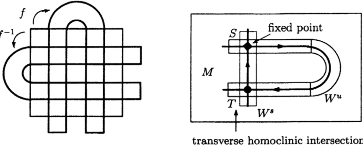
that it is very complicated, actually, chaotic in any small

Figure 5: Horseshoe: Smale’s geometric model (left) and homoclinic intersection (right).

9

Smale Horseshoe

A homeomorphism $f$ : $MO$ of a topological space $M$ is said to admit a horseshoe if there

exist

an

$f$-invariant Cantor subset $J\subset M$ and

a

homeomorphism $Jarrow\Sigma$ that transfers

$f$ : J $O$ to the standard symbolic dynamics $\sigma$ : $\Sigma O$, where $\Sigma$ $:=\{0,1\}^{Z}$ is the topological

space ofbi-infinite sequences of$0$’s and l’s, and $\sigma$ is the shift map

on

$\Sigma$

.

This abstract

sense

of horseshoe

can

be realized by Smale’s famous geometric model of

a

horseshoe-like figure

(see Figure 5, left) [19, 18]. The existence of

a

horseshoe gives evidence of chaos such

as

the positivity of topological entropy and the exponential growth of the number of periodic

points

as

the period tends to infinity, and

so

on.

When $f$ : $MO$ is

a

diffeomorphism of

a

differentiable manifold $M$, the existence of a horseshoe is usually established through the existence ofa transversehomoclinic intersection of stable and unstable manifolds (see Figure 5, right) [20, 18]. This scenario will be applied

to the Painlev\’e dynamics in a neighborhood ofa Riccati curve.

10

Main Result

Let $\gamma\in\pi_{1}(Z, z)$ be a non-elementary loop and

assume

that $\kappa\in H_{0}^{x}$

as

in Section 8. If the

M\"obius transformation $\gamma_{*}$ : $\mathcal{E}_{z}(\kappa)O$ is hyperbolic, then it admits exactly two flxed points,

oneofwhich, say $P$, is expanding at dilationrate $\mu=\mu(\gamma)$ and the other, say $Q$, is attracting

at dilation rate $\mu^{-1}$ for some _$|\mu|>1$

.

Notice that $P$and $Q$

are

saddle fixed pointsat dilation

rates $\mu^{\pm 1}$ of the map

$\gamma_{*}:$ $\mathcal{M}_{z}(\kappa)O$, sincethis map is area-preservingwith respect to the

area

form $\omega_{z}(\kappa)$

.

Thus one can speak of the stable

curve

$W^{s}$ through $P$ and the unstable

curve

$W^{u}$ through $Q$ ofthe map $\gamma_{*}:\mathcal{M}_{z}(\kappa)$ O. Here we remark that $\mathcal{E}_{z}(\kappa)$ is the unstable

curve

through $P$ and at the

same

time the stable

curve

through $Q$

.

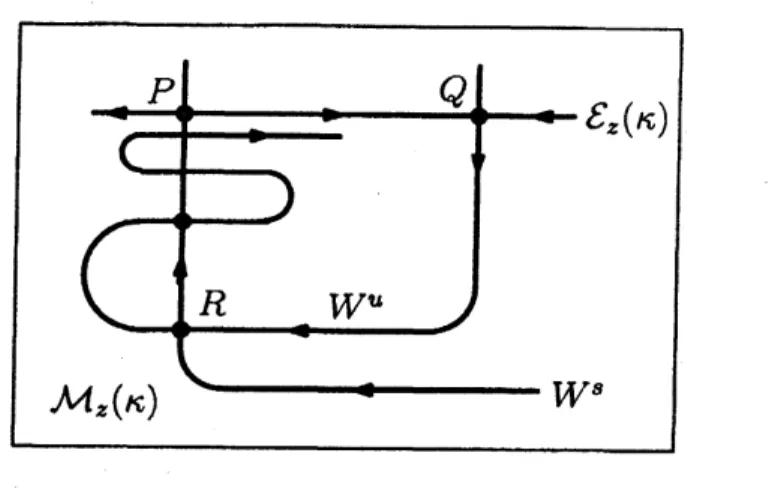
In order to

assure

the presence

of a horseshoe, it is important to

as

$k$ when $W^{\epsilon}$ and $W$“ have a transverse intersection (see

Figure 6). An

answer

to this question is given by the following.

Result 4 For any non-elementary loop $\gamma\in\pi_{1}(Z, z)$ there exists a nontrivial entire

function

$\phi_{\gamma}$ : $H_{0}arrow \mathbb{C}$ such that

if

$\kappa\in H_{0}^{x}\cap\phi_{\gamma}^{-1}(\mathbb{C}\backslash [-1,1])$ , then

$P$ $Q$

$\mathcal{E}_{z}(\kappa)$

R $W^{u}$

$\mathcal{M}_{z}(\kappa)$ $W^{8}$

Figure 6: transverse intersection of the stable and unstable

curves

(2) the stable and unstable

curves

$W^{\theta}$ and _$W^{u}$ have a tmnsverse

intersection; and

(3) there exists an $N\in N$ such that $\gamma_{*}^{N}$ : _{$\mathcal{M}_{z}(\kappa)O$} admits a Smale horseshoe

in any small

neighborhood

_of

the Riccati

curve

$\mathcal{E}_{z}(\kappa)_{f}$ where $N$ depends on the neighborhood

chosen.

Here $\phi_{\gamma}$ being nontrivial

means

that it is not a

constant

_function

urith value in [-1, 1]. The

function

$\phi_{\gamma}(\kappa)$ is computable

once

the loop

$\gamma$ is given explicitly.

This result may fail if $\kappa\in H_{0}^{x}\cap\phi_{\gamma}^{-1}([-1,1])$, but this exceptional subset is very tiny,

being at most of real codimension

one

in $H_{0}^{x}$, since $\phi_{\gamma}$ is anontrivial entire function. In this

sense

the result holds for almost all parameters $\kappa\in H_{0}^{x}$.

Example 5 We illustrate the function $\phi_{\gamma}(\kappa)$ for two loops.

(1) Aneight-figured loop $e_{ij}$ is a loop conjugate to the loop $\gamma_{i}\gamma_{j}^{-1}$ for a cyclicpermutation

$(i,j, k)$ of (1,2, 3)

as

_{in Figure 7 (left). If} $\gamma$ is an eight-figured loop $t_{ij}$, then $\phi_{\gamma}(\kappa)=\cos\pi(\kappa_{i}-\kappa_{k})-\cos\pi(\kappa_{i}+\kappa_{k})-\cos\pi(\kappa_{j}-\kappa_{4})$

.

(2) A Pochhammer loop $\wp_{ij}$ is a loop conjugate to $[\gamma_{i}, \gamma_{j}^{-1}]=\gamma_{i}\gamma_{j}^{-1}\gamma_{i}^{-1}\gamma_{j}$ for

a

cyclic

permutation $(i,j, k)$ of _(1,2,₃₎

as

_{in Figure 7 (right). If}$\gamma$ is

a

Pochhammer loop

$\wp_{ij}$,

$\phi_{\gamma}(\kappa)=2-cos2\pi\kappa_{1}-\cos 2\pi\kappa_{2}-\cos 2\pi\kappa_{3}-\cos 2\pi\kappa_{4}$

$+\cos 2\pi(\kappa_{1}+\kappa_{2})+\cos 2\pi(\kappa_{2}+\kappa_{3})+\cos 2\pi(\kappa_{3}+\kappa_{1})$.

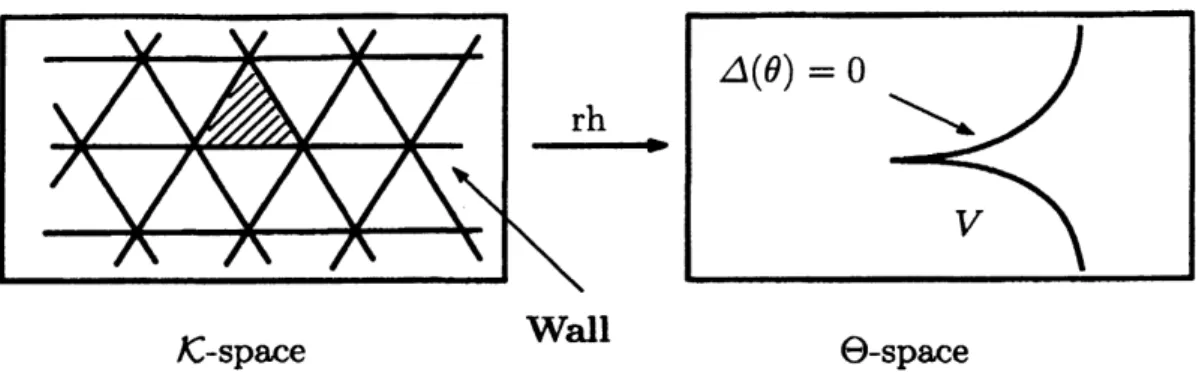
$\mathcal{K}$-space Wall $\ominus$-space

Figure 8: The Riemann-Hilbert correspondence in the parameter level

So

far

we

have restricted

our

attention to the stratum $\mathcal{K}(A_{1})$ for the $s$ake of simplicity. There

are

similar results for the other strata. Result 4 will be shown in [11].

11

Riemann-Hilbert

Correspondence

Result 4 is established, not directly

on

themoduli space $\mathcal{M}_{z}(\kappa)$, butby passing to

a

character

variety $S(\theta)$ through the Riemann-Hilbert correspondence [6, 7, 8, 10],

RH$z,\kappa$ :

$\mathcal{M}_{z}(\kappa)arrow S(\theta)$, $Q\mapsto\rho$, with $\theta=$ rh$(\kappa)$

.

(5)

Here the character varieties for Painlev\’e VI

can

be realized

as a

four-parameter family

of complex affine cubic surfaces $S(\theta)$ parametrized by $\theta\in\Theta$ $:=\mathbb{C}_{\theta}^{4}$ and rh : $\mathcal{K}arrow\Theta$ is

a

holomorphic map that is abranched$W(D_{4}^{(1)})$-covering ramifying alongWall (the unionofall

reflection hyperplanes) andmapping it onto the discriminant locus $V$ $:=\{\theta\in\Theta : \Delta(\theta)=0\}$

of the cubics (see Figure 8). A fUndamental fact for the map (5) is the following.

Theorem 6 ([6, 7, 8])

_If

$\kappa\in \mathcal{K}(*)$ then the chamcter variety $S(\theta)$ unth $\theta=$ rh$(\kappa)$ has

simple singularities

_of

Dynkin $type*and$ the Riemann-Hilbert comespondence (5) is a proper

$su\dot{\eta}ective$ holomorphic map that is

an

analytic minimal resolution

of

singularities.

Take

an

algebraicminimaldesingularization$\varphi:\tilde{S}(\theta)arrow S(\theta)$

.

Then the Riemann-Hilbert

correspondence (5) uniquely lifts to a biholomorphism $\overline{RH}_{z_{2}\kappa}$ : $\mathcal{M}_{z}(\kappa)arrow\tilde{S}(\theta)$ such that

$\mathcal{M}_{z}(\kappa)\underline{\overline{RH}_{z.narrow}}\tilde{S}(\theta)$

$\Vert$ $\downarrow\varphi$

$\mathcal{M}_{z}(\kappa)\underline{R}H_{l\hslash}-,arrow S(\theta)$

is commutative. The lifted Riemann-Hilbert correspondence $\overline{RH}_{z,\kappa}$ maps the Riccati

lo-cus

$\mathcal{E}_{z}(\kappa)\subset \mathcal{M}_{z}(\kappa)$ isomorphically onto the exceptional set $\mathcal{E}(\theta)\subset\overline{S}(\theta)$ of the algebraic

resolution $\varphi$

.

The cubic surface $S(\theta)$ has a natural area-form, that is, the Poincar\’e residue

where $x=(x_{1},x_{2}, x_{3})$ is the standard coordinates of $\mathbb{C}_{x}^{3}$ and $f(x, \theta)=0$ is the defining

equation of the surface $S(\underline{\theta})$ in $\mathbb{C}_{x}^{3}$

.

The Poincar\’e residue

$\omega(\theta)$ lifts to

a

holomorphic

area-form $\tilde{\omega}(\theta)$ $:=\varphi^{*}\omega(\theta)$ on $S(\theta)$, with respect to which the biholomorphism RH

$z_{1}\kappa$ is

area-preserving [9]. The monodromy map $\gamma_{*}:(\mathcal{M}_{z}(\kappa), \omega_{z}(\kappa))O$ is strictly conjugated to

an

automorphism $\sigma$ : $(\tilde{S}(\theta),\tilde{\omega}(\theta))O$, which in tum

can

be extended to a birational map

on

the

natural compactification of $\tilde{S}(\theta)$

.

We then apply the ergodic theory of birational maps on compact surfaces [1, 2, 5, 4] to the last map in order to establish

our

main result.

12

Ergodic Theory

Let $\gamma\in\pi_{1}(Z, z)$ be

a

non-elementary loop. For the monodromy map _{$\gamma_{*}:\mathcal{M}_{z}(\kappa)O$} the

“recurrent”

dynamics takes place only away from infinity, where the vertical leaves $\mathcal{Y}_{z}(\kappa)$

are

thought of

as

the points at infinity in $\mathcal{M}_{t}(\kappa)$

.

Namely the non-wandering set $\Omega_{\gamma}(\kappa)$ of

$\gamma_{*}$ is compact in $\mathcal{M}_{z}(\kappa)$

.

Under the interations of

$\gamma_{*}$, the trajectory of each initial point

$Q\in \mathcal{M}_{t}(\kappa)\backslash \Omega_{\gamma}(\kappa)$ tends to in$finity\mathcal{Y}_{z}(\kappa)$ very rapidly.

The topological entropy $h_{top}(\gamma)$ ofthe map$\gamma_{*}:\Omega_{\gamma}(\kappa)O$ is positive, being represented

as

$h_{top}(\gamma)=\log\lambda(\gamma)$, $\lambda(\gamma)\geq 3+2\sqrt{2}$,

where $\lambda(\gamma)$ is

a

number called the dynamical degree of

$\gamma$, which depends

on

$\gamma$ but is

inde-pendent of $\kappa$

.

There exists a unique

$\gamma_{*}$-invariant probability measure $\mu_{\gamma}=\mu_{\gamma}(\kappa)$, with its

support in $\Omega_{\gamma}(\kappa)$, that is mixing, hyperbolic of saddle type, and of maximal entropy. There

are

positive (1, 1)-currents $\mu_{\gamma}^{\pm}$

on

$\mathcal{M}_{z}(\kappa)$, called thestable and unstable currents, such that

$\gamma_{*}^{\pm 1}\mu_{\gamma}^{\pm}=\lambda(\gamma)\mu_{\gamma}^{\pm}$ and the probability

measure

$\mu_{\gamma}$ is given by the wedge product

$\mu_{\gamma}=\mu_{\gamma}^{+}\wedge\mu_{\overline{\gamma}}$, (6)

where the currents $\mu_{\gamma}^{\pm}$ have continuous potentials so that the wedge product is well defined.

The $s$addle periodic points of $\gamma_{*}$

are

dense in _{$supp\mu_{\gamma}$} and the

measure

is also represented

as

$\mu_{\gamma}=\lim_{narrow\infty}\frac{1}{\lambda(\gamma)^{n}}\sum_{p}\delta_{p}$ (weak limit),

where the

sum

is taken

over

all saddle points ofperiod $n$ and $\delta_{p}$ is the Dirac

mass

at _$p$

.

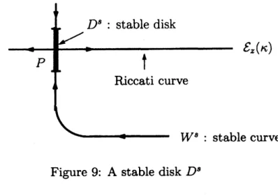
Let $D^{s}\subset W^{\epsilon}$ be

a

stable disk centered at _{$P\in \mathcal{E}_{z}(\kappa)$} (see Figures 6 and 9). Similarly let

$D^{u}\subset W^{u}$ be

an

unstable disk centered at $Q\in \mathcal{E}_{z}(\kappa)$. Then there exist positive constants $c^{\pm}>0$ such that

one

has _weak convergence of_currents

$\lim_{narrow\infty}\frac{1}{\lambda(\gamma)^{n}}[\gamma_{*}^{\mp n}D^{s/u}]=c^{\pm}\mu_{\gamma}^{\pm}$ ,

where $[D]$ denotes the current of integration defined by $\langle[D],$ $v\rangle$ _{$:= \int_{D}v$} for

a

test form

$v$

.

Thus the wedge product in (6) represents the geometric intersections of the stable and

unstable

curves

$W^{s/u}$

.

Then

some

geometric structures of the invariant

measure

$\mu_{\gamma}$ lead to

Figure 9: A stable disk $D^{8}$

13

Concluding

Remark

There are two classes of classical special solutions to the sixth Painlev\’e equation;

one

is the class of Riccati solutions discussed in this paper and the other is that of algebraic solutions

(see e.g. [12, 14, 17, 21]). Here

a

solution of the first class

can

be characterized in terms of

a compact one-dimensional algebraic subset (a curve) in $\mathcal{M}_{z}(\kappa)$ invariant by the nonlinear

monodromy map along every loop, while

a

solution ofthe second class

can

be characterized

by a compact zerodimensional algebraic subset (a set of finite points) enjoying the

same

invariance property [10]. Perhaps the method in this paper could also be applied to

a

solution ofthe second class in order to reveal the presence of chaos around it.

A closely related topic is the non-integrability test for a Hamiltonian system in terms

of differential Galois theory developed in [16], with

an

application to the second Painlev\’e

equation around

a

rational solution [15]. We hope that our dynamical approach would lead

to a deeper result

as

to the “complexity” ofPainlev\’e equations.

References

[1] E. Bedford and J. Diller, Energy and invaiiant

meas

ures

for birational

s

urface maps,

Duke Math. J. 128 (2005), no. 2, 331-368.

[2] E. Bedford, M. Lyubich and J. Smillie, Polynomial diffeomorphisms of $\mathbb{C}^{2}$

.

IV: The

measure ofmaximal entropyand laminax currents. Invent. Math $\dot{1}12$ (1993), 77-125.

[3] S. Cantat and F. Loray, Holomorphic dynamics} Painlev\’e VI equation and character

varieties, e-Print arXiv: 0711. 1579 (2007).

[4] R. Dujardin, Laminar

c

urrents and birationaldynamics, Duke Math. J. 131 (2006),

no.

2, 219-247.

[5] J. Diller and C. Favre, Dynamics of bimeromorphic maps ofsurfaces, Amer. J. Math.

[6] M. Inaba, K. Iwasaki and M.-H. Saito, Dynamics of the sixth Painlev\’e equation,

Th\’eories asymptotiques et \’equations de Painlev\’e, S\’eminaires et Congr\‘es 14, (2006),

103-167.

[7] M. Inaba, K. Iwasaki and M.-H. Saito, Moduli ofstableparabolic connections,

Riemann-HilbertcorrespondenceandgeometryofPainlev\’eequation oftypeVI. PartI, Publ. Res. Inst. Math. Sci. 42 (2006), no. 4, 987-1089.

[8] M. Inaba, K. IwasakiandM.-H. Saito, Moduliofstableparabolicconnections,

Riemann-Hilbert correspondence

an

d geometry ofPainlev\’e equation oftype VI. Part II, Adv.

Stud. Pure Math., 45 (2006), 387-432.

[9] K. Iwasaki, An area-preserving action ofthe modular group

on

cubic surfaces

an

d the

Painlev\’e VI equation, Comm. Math. Phys. 242 (1-2) (2003),

185-219.

[10] K. Iwasaki, Finite branch solutions to Painlev\’e VI around

a

fixed singularpoint, Adv.

Math., 217 (2008), no. 5, 1889-1934.

[11] K. Iwasaki, SmaJe in Painlev\’e around Gauss, in preparation.

[12] K. Iwasaki, On algebraic solutions to Painlev\’e VI, to appear in RIMS Kokyuroku

Bessatsu, e-Print arXiv: 0809.1482 (2008).

[13] K. Iwasaki and T. Uehara, An ergodic study ofPainlev\’e VI, Math. Ann., 338 (2007),

no.

2, 295-345.

[14] O. Lisovyy and Y. Tykhyy, Algebraic solutions of the sixth Painlev\’e equation, e-Print

arXiv: 0809.4873vl (2008).

[15] J.J. Morales-Ruiz, A remark about the Painlev\’e transcendents, Th6oriesasymptotiques

et \’equations de Painlev\’e, S\’eminaires et Congr\‘es 14 (2006), 229-235.

[16] J.J. Morales-Ruiz and J.-P. Ramis, Galoisian obstructions to integrability of

Hamilto-nian systems, Methods and Applications ofAnalysis 8 (2001),

no.

1, 33-96.

[17] K. Okamoto, Studyof thePainlev\’eequations I, sixth Painlev\’eequation $P_{VI}$,Ann. Math.

Pura Appl. (4) 146 (1987), 337-381.

[18] C. Robinson, Dynamical systems–stability, symbolic dynamics, and chaos $-2i\iota d$ed.,

CRC Press, 1999.

[19] S. Smale, Diffeomorphisms with many periodic points, Differential and Combinatorial

Topology, pp. 63-80, Princeton Univ. Press, Princeton, 1965.

[20] S. Smale, Differentiable dynamicalsystems, Bull. Amer. Math. Soc. 73 (1967),

747-817.

[21] H. Watanabe, Birational canonical transformations and classical solutions of the sixth