Functional differential
equations
of
a
type
similar to
$f’(\mathrm{x})=2f(2x +1)$
$-2f(2x-1)$
and
its application.
大阪教育大学
米田
劉
(Tsuyoshi Yoneda)
Department of
Mathematics
Osaka
Kyoiku
University
Frederickson
$\int_{\mathrm{L}}1$],
[2}
(1971)
investigated functional-differential equations of
ad-vanced
type
(0.])1
$f’(x)=af(\lambda x)+bf(x)$
,
where A
$>1$
,
and provided several
properties
of
solutions.
Kato
and McLeod
[4]
(1971)
and
Kato [
$3_{d}1$(1972)
studied
asymptotic behavior
of solutions of (0.1).
By
using
another
method, the
author
[6]
constructed one of the solutions
for
the
equation
(0.2)
$\{$$f’(x)=af(2x)’$
.
$x$
$\in \mathbb{R}$$=l-\backslash \infty,$
$+\infty \mathrm{I},$,
$f\acute{(}0)=0$
,
where
$a$
is
a
constant with
$a$
$\neq 0$
. The
solution
is
not unique. If
$f$
is
a
solution,
then
a
constant
times
$f$
is
also a solution.
Our solutions are
infinitely differen liable
and bounded on
R. In
$\mathrm{I}6\underline{1}$,
the
author gave
the
graph of
the
solution
$f(x,1$
of
(0.2)
with
$a$
$=4$
(Figure 1).
In
this
paper,
we
construct
a solution
for the
functional
differential
equation;
(0.3)
$f^{(n\}}(x)= \lambda^{n\dotplus 1}\sum_{j}cj\mathcal{B}_{j}^{n}\sum_{t=\iota}^{n}\hat,(-1)^{1}$$(\begin{array}{l}nt\end{array})f\mathrm{f}\lambda x-\backslash \frac{l-n/2+nk_{j}}{\beta_{j}})$,
where
$\nabla_{j}\angle-c_{j}=1_{j}\sum_{j}c_{\mathrm{i}}\beta;<\infty,c_{j}\geq 0$
,
$\inf_{j}\beta_{j}>0$
,
$\sup_{j}|k_{j}$
.
[
$<\infty$
and
$\sum_{j}$1
$\mathrm{s}$finite
sum
or
infinite
sum.
The solution
is
unique
in
$L^{1}(\mathbb{R}\rangle$up to
a
multiplicative constant
and
it is in
$C_{comp}^{\infty}(\mathrm{R})$ $\cap L^{1}(\mathbb{R})$.
(Some
special
cases
were treated in [5].) We
also
give
the
method
of
cal culating
numerical
data.
For example, the following is
a
special
case
of
(0.3).
$(0,4)$
$f^{J}(x,\}=4f(2x,1 -4f(2x-1)$
.
The graph of the
solution of (0.4) is in
Figure 2, which
is
a
component of
the graph
of
Figure
1.
Our main result
is
as
follows.
FIGURE
2. The solution
of
$(0.4\grave{J}$.
Theorem
0.1. The equation
$(0.3)\backslash$has
a
unique
solution
in
$L^{1}\{\mathbb{R}$)
up to
a
multi-plicative constant and it is in
$C_{\mathrm{c}omp}^{\infty}(\mathbb{R})${T
$L^{1}(\mathrm{i}\mathrm{R})$.
We
give
some
examples of (0.3).
$(\mathrm{E}1)\backslash f^{t}(x)=2f(2x+1)-2f(2x-1)$
,
(E2)
$f’(x)=16f(4x)-16f(4x -1)$ ,
(E3)
$f^{\mathit{1}}(x)=(9/4)f(3x/2\}-\{9/4)f(3x/2-1)$
,
(E1)
$f’(x)=3;(.2x)-2f\zeta 2x$
- $1$)
$-f(2x-2)$
,
(E5)
$f^{J}(x)=3f(2x)-3f(2x-1)+f(2x-2)-f_{\backslash }^{(}2x-3)_{7}$
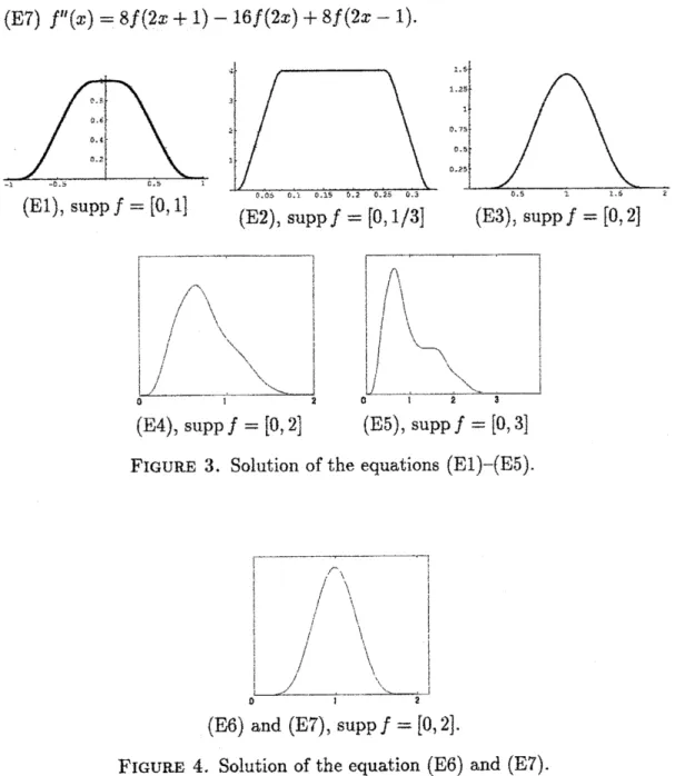
(E7)
$\mathrm{f}"(\mathrm{x})=8f(2x+1)$
$-16f(2x)+8f\zeta 2x-1)$
.
(E1},
$\mathrm{s}\mathrm{u}\mathrm{p}\mathrm{p}f=[0, 1]$(E2),
$\mathrm{s}\mathrm{u}\mathrm{p}\mathrm{p}/=[0, 1/3]$(E3),
$\mathrm{s}\mathrm{u}\mathrm{p}\mathrm{p}f=[0,2]$$\overline{0|,\prime}///’/’/^{l}/’\backslash \wedge\frac{\backslash \backslash |\backslash _{4}\backslash _{\backslash 1_{\mathrm{I}}^{\mathrm{t}}\backslash \backslash 1}\backslash \backslash \sim|}{12}$
(E4),
$\mathrm{s}\mathrm{u}\mathrm{p}\mathrm{p}f=[0_{;}2]$(E5),
$\mathrm{s}\mathrm{u}\mathrm{p}\mathrm{p}f=\mathrm{l}\mathrm{r}_{\mathrm{Q}}$,
$3_{\mathit{1}}^{1}$FIGURE 3. Solution of the
equations
(E1) (E5),
$0 \{|||\mathrm{t}|_{1}||’ \mathrm{m}^{i}\frac{/^{l}\backslash j/_{11\backslash _{1}}^{/^{\Gamma_{\backslash }}\backslash }|_{1}\prime \mathfrak{l}\backslash \backslash \backslash \backslash \backslash \backslash \neg|}{12}//\cdot$
(E6)
and
(E7),
$\mathrm{s}\mathrm{u}\mathrm{p}\mathrm{p}f=[0,2]$.
FIGURE
4. Solution
of
the equation
(E6) and (E7).
We
have
considered
application of the function
(E1)
by
using “Quark theory”
es-tablished
by
ff.Trebel.
Next section, we
introduce
the
result
of
application, This
application is
considered with Yoshihiro Sawano
who belongs to Tokyo University.
1.
RESULT
OF
APPLICATION
Let
$0<p$
,
$q\leq\infty$
and
$s>\sigma_{\mathrm{p}}$.
$B_{pq}^{\delta}(\mathbb{R})$is
a set
of Schwartz
distributions
$f$
for
which
$f$
can
be
written
as
(1.1)
$f= \sum_{\beta\in \mathrm{N}_{\mathrm{O}}^{d}}\sum_{\nu=0}^{\infty}\sum_{m\in \mathrm{Z}^{d}}\lambda_{\nu,m}^{9}.l2^{-\nu(s-d/p)}(2^{p}x-m)^{\beta}\phi(2^{\nu}x-m)$where,
the finction
$\phi$satisfies
$\phi’(x)=2\phi(2x+1)-2\phi(2x-1)$
.
Theorem 1.1. The equation
$f^{l}(x)=f(x-1)$
can
solve
explicty with
following
initid data
$f|_{[0_{1}\mathrm{I}]}=( \sum_{\beta\in \mathrm{f}\backslash \mathrm{i}_{0}}\sum_{\nu\in \mathrm{E}_{0}},\sum_{m\in_{arrow:q_{\nu_{\mathrm{t}}m}\mathrm{n}[0,\mathrm{x}]\neq\emptyset}^{m}}\lambda_{\nu,m}^{\beta}2^{-\nu(s-d/p)}(2^{\nu}x-m)^{\beta}\phi(2^{\nu}x-m\rangle)oe\in \mathrm{f}^{0,1}]$
The solution
$f|\mathfrak{t}1,2_{\mathrm{J}}^{1}$can
be
written
as
follows;
$f(x)$
$=$
$f(1)+ \sum\sum$
$\beta\in \mathrm{N}_{0}\nu\in 1\forall 0m\in \mathbb{Z}j\sum_{q_{\nu,m}\cap[0,1]\neq \mathfrak{g}}2^{-\nu}\lambda_{\nu_{\mathrm{J}}m}^{\beta}\oint_{\nu,m}^{*}(x -1)$
$+( \oint_{\mathrm{P}_{\vee}}. x^{\beta}\phi(x)dx)\sum_{\nu\in \mathrm{R}^{1_{\mathrm{Q}}}}\sum_{\mathrm{z}\leq 2^{\nu}}(\sum_{t=0}^{m-2}\lambda_{\nu,t}^{0}2^{-\nu)}\phi(2^{\nu}x-m-1)$
.
where
$\phi_{\nu,m}^{\beta*}(x)$
$:=$
$( \sum_{\tau\subset\emptyset}^{\beta}(-1)^{\gamma}$$(\begin{array}{l}\beta\gamma\end{array})$$(2^{\nu}x-m)^{\beta-\gamma}I_{\gamma}(\phi(2^{\nu}x-m)))$
$-2-p(s- \frac{\#}{\mathrm{p}})_{(}[_{-\sim}\overline{|\mathfrak{l}}dx^{\beta}\phi(x)$
&)
$\sum_{t=2}^{\infty}\phi(2^{\nu}(x-l)-m)$
,
$I_{\beta}( \phi)(x)=\sum_{j_{\theta+1}=0}^{\infty}\sum_{I\rho=0}^{\infty}-,\cdot$
. .
$\sum_{j_{1}=0}^{\infty}2^{\frac{\beta[\beta_{\mathrm{T}^{1}}1]}{2}}\phi(\frac{x-2^{\beta+1}+1}{\mathfrak{X}^{+1}}-\sum_{\gamma=1}^{\beta+\mathrm{I}}\frac{j_{\gamma}}{2^{\gamma-1}})$and
$I_{0}( \phi)(x)=\sum_{\mathrm{j}=0}^{\infty}\phi(\frac{x-1-2j}{2})$
.
2.
ACKNOWLBDGEMENT
REFERENCES
[1] P.
0
Frederickson,
Global
solutions
to certain nonlinear
functional
differential
equations.
J.
Math. Anal.
Appl.
33
(1971),
355-358.
[2] P.
O.
Frederickson,
Diricklet
series
solutions
for
certain
functional differential
equations.
Japan-United
States Seminar on
Ordinary
Differential
and
Functional Equations
(Kyoto,
1971),
249-254.
Lecture Notes
in
Math.,
Vol.
243,
Springer,
Berl
in,
1971,
[3]
T. Kate,
Asymptotic behavior
of
solutions
of
the
functional
differential
equation
$y’(x\rangle=$
$\mathrm{a}\mathrm{y}(\mathrm{X}\mathrm{x})$