Application of empirical likelihood method to time series model (A Bayesian Approach to Statistical Inference and Its Related Topics)

(1)

Application of empirical

likelihood

method

to

time series

model

早稲田大学・国際教養学部小方浩明 (HiroakiOgata)

School

of

Intemational

Liberal Studies,

Waseda University

1 Introduction

Empirical likelihood method is

one

of the nonparametric methods for statistical

in-ference proposed by Owen (1988, 1990). It is shown thatempirical likelihood ratio is

asymptotically chi-square distributed and used for constructing confidence regions for

thesample mean, for

a

class ofM-estimatesthat includes quantile, andfor differentiable

statistical functionals. $Emp\ddot{m}cal$

likelihood

has been studied extensively in the

litera-ture because ofits generality and effectiveness. We

can

name many

applications, such

as

general estimating equations (Qin and Lawless (1994)), regression models (Owen (1991), Chen (1993, 1994)$)$, biased sample models (Qin (1993)), etc. Although

em-pirical likelihood method has been smdied by

many

authors, it

seems

to have been

investigated mainly under i.i.$d$

.

setting. For dependent observations, Kitamura (1997)

developedblockwise empiricallikelihoodfor estimatingequations and for smooth

func-tions of

means.

Monti (1997) applied the $emp\ddot{m}cal$ likelihood method to dependent

observations,essentially undercircular Gaussian assumption, using

a

spectral method.

In this resume,

we

introduce

some

parts of

our

previous works

on

the

extension

of

the $emp\ddot{m}cal$ likelihood method to non-Gaussian stationary

processes

by

use

of

spec-tral approach. In Section 2,

_we

deal with non-Gaussian scalar stationary

processes.

Motivated by the Whittle likelihood,

we

introduce estimating functions for dependent observations and derive the asymptotic distribution of the $emp\ddot{m}cal$ likelihood ratio.

In Section 3, we extend the setting to non-Gaussian vector stationary

processes.

The method of fitting parametric model is also considered and by choosing this parametric

function properly,we

can

considertheestimation problem of theautocorrelation,which

is

one

of the most important indices for time series analysis. In Section4,

we

study

an

application of themethod with Cressie-Read power-divergencestatistic (CR statistic)to

non-Gaussian vector stationary

processes.

CR method is

more

general than $emp\ddot{m}cal$

likelihood method. In this setting,

we

consider the problem of testing, too. Various

(2)

2 Empirical

likelihood

method for

_non-Gaussian

_scalar

stationary

processes

We consider

a scalar-valued

linear

process

$\{X(t);t\in R\}$, generated

as

$X(t)= \sum_{j=0}^{\infty}G(])e(t-j)$, $t\in R$, (1)

where $\{e(t)\}$ is

a

sequence of random variables satisfying _{$E\{e(t)\}=0$} and _{$E\{e(t)e(s)\}=$}

$\delta(t, s)\sigma^{2}$,with_{$\sigma^{2}>0,G(j)$}’s

are

constants,and the

$X,e$and$G$

are

allreal. If$\sum_{j=0}^{\infty}G(])^{2}<$

$\infty$ (this condition isassumed throughout inthis section),the

process

$\{X(t)\}$ is

a

second-order

stationary process,

_{and has the spectral}_{density function}

$g( \omega)=\frac{\sigma^{2}}{2\pi}|\sum_{j=0}^{\infty}G(])e^{-i\omega j}|^{2}$, $-\pi<\omega\leq\pi$. (2)

For the stretch $X(t),$ $t=1,$$\ldots,$ $T$,

we

denote by $1_{T}(\omega)$,the periodogram; namely

$I_{T}( \omega)=\frac{1}{2\pi T}|d_{T}(\omega)|^{2}$, where _{$d_{T}( \omega)=\sum_{t=1}^{T}X(t)\exp\{-i\omega t\}$}

$-\pi<\omega\leq\pi$

.

We setdown the following assumptions.

Assumption

2.1.

(i) $\{X(t)\}$ is strictly stationarywithall

of

whose moments exist.

(ii) _The_joint _{k-th order cumulant} $c_{X^{k}}(u_{1}, \ldots, u_{k-1})$

of

$X(t),X(t+u_{1}),$ _{$\ldots,X(t+u_{k-1})$}

satisfies

$u_{1} \ldots..u=-\infty\sum_{k- 1}^{\infty}(1+|u_{j}|)|c_{X^{k}}(u_{1}, \ldots, u_{k-1})|<\infty$

for

$j=1,$ $\ldots,k-1$ andany $k,$ $k=2,3,$

$\ldots$ .

Assumption

2.2.

For thesequence $\{C_{k}\}$

defined

by

$C_{k}= \sum_{u_{1},\ldots,u_{k}=-\infty}^{\infty}|c_{X^{k}}(u_{1}, \ldots, u_{k-1})|$,

itholds that

$\sum_{k=1}^{\infty}C_{k}z^{k}/k!<\infty$

(3)

Denote by $g_{k}(\omega_{1}, \ldots, \omega_{k-1})$, the k-th order spectral density of the process _$\{X(t)\}$;

namely

$g_{k}( \omega_{1}, \ldots, \omega_{k-1})=(2\pi)^{-k+1}\sum_{u_{1},\ldots,u_{k}=-\infty}^{\infty}c_{X^{k}}(u_{1}, \ldots, u_{k-1})\exp(-i\sum_{j=1}^{k-1}u_{j}\omega_{j})$

.

Henceforth

we

assume

that spectral density depends

on an

unknown parameter $\theta$

in this section: thus $g(\omega)=g(\omega, \theta),$ $g_{k}(\omega_{1}, \ldots,\omega_{k-1})=g_{k}(\omega_{1}, \ldots,\omega_{k-1};\theta)$

.

In what

follows,

we

state thefundamental results

on

periodogram.

Lemma

2.1.

Let $\{X(t)\}$ satisfy Assumption 2.1. Let $A(\omega),$$-\pi<\omega\leq\pi$ be

a

q-dimensional vector valuedcontinuous function, satisfying $A(\omega)=A(-\omega)$

.

Then

$T^{-1/2} \sum_{t=1}^{T}A(\lambda_{t})\{I_{T}(\lambda_{t})-El_{T}(\lambda_{t})\}arrow dN(O,\Sigma_{1})$ $(Tarrow\infty)$,

where $\lambda_{t}=2\pi t/T$ and

$\Sigma_{1}$ $=$ $\frac{1}{2\pi}\int_{-\pi}^{\pi}\int_{-\pi}A(\omega_{1})A(\omega_{2})’g_{4}(\omega_{1}, -\omega_{1},\omega_{2})d\omega_{1}d\omega_{2}$

$+ \frac{1}{\pi}\int_{-\pi}A(\omega)A(\omega)’g(\omega)^{2}d\omega$

.

Lemma

2.2.

Underthe

same

assumption

as

in Lemma 2.1, itholds that

$T^{-1} \sum_{t=1}^{T}\{A(\lambda_{t})I_{T}(\lambda_{t})\}\{A(\lambda_{t})I_{T}(\lambda_{t})\}’arrow p\Sigma_{2}$ $(Tarrow\infty)$,

where

$\Sigma_{2}$ $=$ $\frac{1}{\pi}\int_{-\pi}^{\pi}A(\omega)A(\omega)’g(\omega)^{2}d\omega$

.

$Emp\ddot{m}cal$ likelihood allows

us

to

use

likelihood methods,without assumingthatthe

data

come

from

a

known family ofdistribution. Empiricallikelihood method isbased

on

the nonparametric likelihood

ratio

$R(F)= \prod_{i=1}^{n}np_{i}$ where$F$

is

an

arbitrary distribution

which has probability $p_{i}$

on

the obtained data $X_{i}$

.

We

use

this

ratio

$R(F)$

as

a

basis for

hypothesis testingand confidence intervals.

When we

are

interested in parameter $\theta\in R^{q}$ which satisfies _{$E[m(X,\theta)]=0$}, where

$m(X,\theta)\in R^{q}$ is

a

vector-valued function, called

estimating

function,

we

consider the

empirical likelihoodratio function $R(\theta)$ (defined in (5) below). As

a

test statistic, it is

shownthat $-2\log R(\theta)$ tendstochi-square withdegree offreedom$q$,when$X_{i}$’s

are

i.i.$d$

.

(4)

Here,

we

consider

the

case

of dependent sample. When $\{X(t)\}$ is

a

Gaussian

circu-lar ARMA

process,

Anderson (1977) _showed _{that the} $\log$ likelihood $LL_{c}(\theta)$ for $X=$

$(X(1), \ldots,X(T))’$ _becomes,_disregarding

_a

_constant_term,

$LL_{c}( \theta)=-\sum_{t--1}^{T}\{\log g(\lambda_{t},\theta)+\frac{I_{T}(\lambda_{t})}{g(\lambda_{t},\theta)}\}$,

and that$2I_{T}(\lambda_{t})/g(\lambda_{t}, \theta),$$t=1,$

$\ldots,$ $(T/2)-1$

or

$(T-1)/2$,

are

independentlydistributed,

each with$\chi_{2}^{2}$-distribution, where _{$I_{T}(\lambda_{t})$}is the periodogram of_$X$

and$g(\lambda_{t}, \theta)$ is the

spec-tral density which depends

on an

unknown parameter $\theta$

.

Without the assumption of

circular Gaussian ARMA

process,

it is

known that Anderson’s results hold

asymptot-ically (e.g. Taniguchi and Kakizawa (2000, _Section 7.2.2)). That is, if $\{X(t)\}$ is

an

appropriate

stationary process,

$2I_{T}(\lambda_{t})/g(\lambda_{t},\theta),$ $t=1,$ $\ldots,(T/2)-1$

or

$(T-1)/2$

are

asymptoticallyindependent and asymptotically$\chi_{2}^{2}$-distributed.

Monti (1997) _{applied the spectral approach of this type} _to _the $emp\ddot{m}cal$ likelihood,

andconsidered

an

integral versionof$LL_{c}(\theta)$,whichis called theWhittle likelihood,that

is,

$WL( \theta)\equiv\int_{-\pi}^{\pi}\{\log g(\omega,\theta)+\frac{I_{T}(\omega)}{g(\omega,\theta)}\}d\omega$, (3)

and used$\psi_{t}(\theta)=(\partial/\partial\theta)\{\log g(\lambda_{t},\theta)+I_{T}(\lambda_{t})/g(\lambda_{t}, \theta)\}$

as a

counterpart ofOwen’s _{$m(X,\theta)$}

.

Then,Monti(1997) _{showed that}$-2\log R(\theta)$ tends tochi-square with degree offreedom

$q$

.

However, her proofof the above resultessentially relies

on

Anderson’s results.

In this section, assuming that $\{X(t)\}$ is

a

non-Gaussian scalar stationary process,

we

give therigorousproof ofit. First,

_we

impose thefollowing assumptions.

Assumption

2.3.

$g(\omega, \theta)$ is continuously twice

differentiable

withrespectto$\theta$.

Assumption $2A$

.

_(i) $\theta_{0}$ is the true value

of

a

parameter

of

interest$\theta$

.

(ii) $\theta_{0}$ is innovationfree, thatis,

$f_{-\pi} \frac{\partial}{\partial\theta}\{g(\omega, \theta)\}^{-1}g(\omega,\theta)d\omega|_{\theta=\theta_{0}}=0$

.

(4)

If$\theta$is innovation-free,

$(\partial/\partial\theta)WL(\theta)|_{\theta=\theta_{0}}=0$ becomes

$\int_{-\pi}\frac{\partial}{\partial\theta}\{\frac{I_{T}(\omega)}{g(\omega,\theta)}\}d\omega|_{\theta=\theta_{0}}=0$

andits discriterized version of the lefthandsideis

(5)

Because

it

is

knownthat $E\{I_{T}(\lambda_{t})\}$

converges

to$g(\lambda_{t}, \theta_{0})$,

we

can see

that

$\frac{1}{T}\sum_{t=1}^{T}E[\frac{\partial}{\partial\theta}\{\frac{l_{T}(\lambda_{t})}{g(\lambda_{t},\theta)}\}|_{\theta=h}]arrow 0$

whichmotivates

our

empirical likelihoodratio function $R(\theta)$defined by

$R( \theta)=\max_{w}\{\prod_{t=1}^{T}Tw_{t}|\sum_{t=1}^{T}w_{t}m(\lambda_{t}, \theta)=0,$ $w_{t}\geq 0,$ $\sum_{t=1}^{T}w_{t}=1\}$ , (5)

where $w=(w_{1}, \ldots, w_{T})’$ and

$m( \lambda_{t},\theta)=\frac{\partial}{\partial\theta}\{\frac{l_{T}(\lambda_{t})}{g(\lambda_{t},\theta)}\}$

.

We setdown thefollowing furtherassumption.

Assumption

2.5.

Theprocess $\{e(t)\}$

satisfies

$cum\{e(t_{1}),e(t_{2}),e(t_{3}),e(t_{4})\}=\{\begin{array}{ll}\kappa^{4} (t_{1}=t_{2}=t_{3}=t_{4})0 (otherwise)\end{array}$

Then we get thefollowing theorem.

Theorem

2.1.

Let $\{X(t)\}$ be

a

scalar-valued linear

process

defined

in (1), and

satisff

Assumptions 2.1 $\sim$

2.5.

$Then-2\log R(\theta_{0})arrow\chi_{q}^{2}d$

as

$Tarrow\infty$

.

Using this theorem,

we

can

constmct

a

confidence regions of $\theta$

.

First,

we

choose

a

proper

threshold value $z_{a}$, which is $\alpha$ percentileof$\chi_{q}^{2}$

.

Then

we

calculate $-2\log R(\theta)$ at

divisionpoints

over

the

range

andconstructthe region

$C_{a,T}=\{\theta|-2\log R(\theta)<z_{a}\}$

.

3 Empirical likelihood

method for

non.Gaussian vector

stationary

processes

with fitting

parametric

spectral

model

Consider

a

vector-valued linear

process

$\{X(t);t\in Z\}$ generatedby

$X(t)= \sum_{j=0}^{\infty}G(])e(t-])$, $t\in Z$, (6)

where$X(t)$’shave$s$componentsand$e(t)$’s

are

$s$dimensionalvectorssatisfying$E[e(t)]=$

(6)

$s$ matrices,and the components of _$X,$_$e$ and _$G$

are

all real. If

$\sum_{j=0}^{\infty}$ tr$\{G(])KG(])’\}<\infty$ (this _condition _is _assumed _throughout _in _this _section), _the

_process

_$\{X(t)\}$ _is

_a

second-orderstationary

process

and has the spectral_density _matrix _which _is _expressed

_as

$g( \omega)=\frac{1}{2\pi}k(\omega)Kk(\omega)^{*}$, _{$-\pi<\omega\leq\pi$}

, (7)

where $k( \omega)=\sum_{j=0}^{\infty}G(j)e^{i\omega j}$

.

For the stretch _$X(t),$ $t=1,$

$\ldots,$$T$,

we

denote by $I_{T}(\omega)$,the

periodogram; namely

$I_{T}( \omega)=\frac{1}{(2\pi T)}d_{T}(\omega)d_{T}(\omega)^{*}$, _{$-\pi<\omega\leq\pi$}

.

(8)

where $d_{T}( \omega)=\sum_{t=1}^{T}X(t)e^{-i\omega}$‘. We setdown the following assumptions.

Assumption

3.1.

(i) $\{X(t)\}$ is strictlystationarywith all

of

whose_momentsexist.

$(li)$ Thejoint k-th order cumulant_{$c_{X^{k}}(u_{1}, \ldots, u_{k-1})_{\beta_{1}\beta_{2}..\beta_{k}}ofX(t)_{\beta_{1}},X(t+u_{1})_{\beta_{2}},$} _{$\ldots,X(t+$} $u_{k-1})_{\beta_{k}}$

satisfies

$\sum_{u1\cdots\cdot\cdot u_{k- 1}=-\infty}^{\infty}(1+|u_{j}|)|c_{X^{k}}(u_{1}, \ldots,u_{k-1})_{\beta_{1}..\beta_{k}}|<\infty$ (9)

for

$j=1,$ $\ldots,k-1,\beta_{1},$$\ldots,\beta_{k}=1,$

$\ldots,$$s$andany $k,$ $k=2,3,$$\ldots$

.

Assumption

3.2.

For thesequence $\{C_{k}\}$

defined

by

$C_{k}= \sup_{\beta_{1},\ldots\beta_{k}}\sum_{u_{1},\ldots,u_{k}=-\infty}^{\infty}|c_{X^{i}}(u_{1}, \ldots, u_{k-1})_{\beta_{1}..\beta_{k}}|$,

itholds that

$\sum_{k=1}^{\infty}C_{k}z^{k}/k!<\infty$

for

$z$ in a neighborhood

of

$0$.

We denote by $g_{k}(\omega_{1}, \ldots,\omega_{k-1})_{\beta_{1}..\beta_{k}}$, the k-th order spectral density of the

process

$\{X(t)\}$; namely

$g_{k}( \omega_{1}, \ldots,\omega_{k-1})_{\beta_{1}..\beta_{k}}=(2\pi)^{-k+1}\sum_{ku_{1},\ldots,u=-\infty}^{\infty}c_{X^{\hslash}}(u_{1}, \ldots, u_{k-1})_{\beta_{1}..\beta_{k}}\exp(-i\sum_{j=1}^{k-1}u_{j}\omega_{j})$.

In Section 2,

we

extended the $emp\ddot{m}cal$ likelihood method to non-Gaussian scalar

(7)

apply the method to

non-Gaussian

vector

stationary

processes.

The difference from

Section 2 is not only that

we

deal with vector

processes

but also that

we

use

a

fitting

parametric spectral model insteadofparametrized true spectral density.

For the vector-valued non-Gaussian linear

process

(6) with the true spectral density

matrix $g(\omega)$,

we

fit

a

parametric spectral model $f(\omega,\theta)$with $\theta\in\Theta\subset R^{q}$,to _$g(\omega)$

.

Here $f(\omega, \theta)$

may

be different from $g(\omega)$

.

Consider the multivariateWhittle likelihood

$\int_{-\pi}^{\pi}[\log\det f(\omega,\theta)+ff\{f(\omega,\theta)^{-1}l_{T}(\omega)\}]d\omega$

.

Here,

we

impose

the following assumption

on

the parametric spectral model$f(\omega,\theta)$

.

Assumption

33.

(i) $\Theta$ is

a

compact subset

of

$R^{q}$

.

(ii) $f(\omega, \theta)$ iscontinuouslytwice

differentiable

with respect to$\theta\in\Theta$

.

(iii) $f(\omega,\theta)\in F$

.

Here

9“

istheparametricspectralfamilywhose element isexpressed

$as$

$f( \omega,\theta)=(\sum_{j=0}^{\infty}C_{j}(\theta)e^{ij\omega})\Sigma(\sum_{j=0}^{\infty}C_{j}(\theta)e^{ij\omega})^{*}$ (10)

where $C_{j}(\theta)$ is $s\cross s$matrices,$C_{0}(\theta)$ is $s\cross s$ unitmatrixand$\Sigma$ is

an

_{$s\cross s$}positive

definite

matrix which is independent

_of

$\theta$

.

The above model (10) is the spectral form of the general linear

process

so

this

assump-tion is quitenamral. Notethat theparameter$\theta$does not depend

on

$\Sigma$,whichcorresponds

tothecovariance matrix ofthe

innovation.

Likethis,when$\theta$depends

on

only the

coeffi-ciemparts$C_{j}$and doesnotdepend

on

theinnovationpart$\Sigma$,

we

call$\theta$”$innovation$-free”.

Let $\theta_{0}$be thevalue defined by

$\frac{\partial}{\partial\theta}\int_{-\pi}^{\pi}[\log\det f(\omega,\theta)+\ddagger r\{f(\omega,\theta)^{-1}g(\omega)\}]d\omega|_{\theta=\theta_{0}}=0$, (11)

whichis called the pseudo-true vale of$\theta$

.

We

use

$D(f_{\theta}, g):= \int_{-\pi}[\log\det f(\omega,\theta)+\ddagger r\{f(\omega, \theta)^{-1}g(\omega)\}]d\omega$

as a

disparity

measure

between $f(\omega,\theta)$ and $g(\omega)$,

so

$\theta_{0}$

means

the point minimizing

the $D(f_{\theta}, g)$

.

If $\theta$ is innovation-free, then $J_{-\pi}^{\pi}$log det$f(\omega,\theta)d\omega$ is independent of $\theta$

(Brockwell-Davis (1991,

p.

191). Therefore (11)becomes

(8)

Furthermore,bychoosing$f(\omega, \theta)$ appropriately,$\theta_{0}$

can

show various

important

indices

oftime series model. One ofsuch examples is the autocorrelation,_{which is introduced}

in thefollowing.

Example

3.1.

Denote$\Gamma(\delta)=cov\{X(t), X(t+\delta)\}$ asthe autocovariance matrix

_of

_$X$_with

lag $\delta$

.

Let

us

considerthe linear process

_defined

in (6).

_If

_we

_set

$\theta=(\theta_{11}, \ldots, \theta_{1s}, \ldots\ldots, \theta_{s1}, \ldots,\theta_{ss})’$,

$A(\theta)=[\theta_{s1}\theta_{11}$ $.\cdot.\cdot$ . $\theta_{ss}\theta_{1s})$, and $f(\omega,\theta)=(I-A(\theta)e^{i\delta\omega})^{-1}(l-A(\theta)e^{i\delta\omega})^{-1^{*}}$,

then condition (12) shows

$\sum_{j=1}^{s}A(\theta_{0})_{\beta_{1}j}\int_{-\pi}^{\pi}g(\omega)_{j\beta_{2}}d\omega=\int_{-\pi}e^{i\delta\omega}g(\omega)_{\beta_{2}\beta_{1}}d\omega$ _{$(\beta_{1},\beta_{2}=1, \ldots, s)$}

.

(13)

It is well _{known that the autocovariance and the} _spectral _{density have the following}

relation

$\Gamma(\delta)=\int_{-\pi}^{\pi}e^{i\delta\omega}g(\omega)d\omega$. (14)

From (13) and(14),

we

obtain

$A(\theta_{0})\Gamma(0)=\Gamma(\delta)’$ $\Leftrightarrow$ $A(\theta_{0})=\Gamma(\delta)\Gamma(0)^{-1}$

.

Hence,

_{we can}

_{estimate the} _quantity$\Gamma(\delta)\Gamma(0)^{-1}$ , which is

a

generalized quantity

of

the

usual autocorrelation$\rho(\delta)=\Gamma(\delta)/\Gamma(0)$in scalar

case.

As

a

natural extension from the scalar

case

in Section 2,

_we

define

an

estimating

function $m(\lambda_{t}, \theta)$

as

$m( \lambda_{t},\theta)=\frac{\partial}{\partial\theta}$tr$\{f(\lambda_{t},\theta)^{-1}I_{T}(\lambda_{t})\}$ where $\lambda_{t}=\frac{2\pi t}{T},$ $t=1,$

$\ldots,$ $T$ (15)

according to (12). In addition,

_we

_use

_the $emp\ddot{m}cal$ likelihood ratio function $R(\theta)$

de-fined in (5). Then

we

obtain the following theorem.

Theorem

3.1.

Let$\{X(t)\}$ be thelinearprocess

defined

in (6)satisfying Assumptions

3.1

$- 3.3$

.

Then

(9)

as

$Tarrow\infty$_, where $N$ has

a

q-dimensional stamdard normal distribution and _$A=$

$\Sigma_{4}^{-1/2}\Sigma_{3}^{1/2}$. Here $\Sigma_{3}$ is

$q$ by $q$ matrix whose $(\gamma_{1}, \gamma_{2})$ elementis

$(\Sigma_{3})_{\gamma_{1}\gamma_{2}}$ $=$ $\frac{1}{\pi}\int_{-\pi}^{\pi}tr[g(\omega)\frac{\partial f(\omega,\theta)^{-1}}{\partial\theta_{\gamma_{I}}}|_{\theta=\theta_{0}}g(\omega)\frac{\partial f(\omega,\theta)^{-1}}{\partial\theta_{72}}|_{\theta=h}]d\omega$

$+ \frac{1}{2\pi}\sum_{\beta_{1},\ldots\beta_{4}=1}^{s}\int\int_{-\pi}^{\pi}\frac{\partial f(\omega_{1};\theta)^{\beta_{1}\beta_{2}}}{\partial\theta_{71}}|_{\theta=\phi}\frac{\partial f(\omega_{2};\theta P^{3}\beta_{4}}{\partial\theta_{\gamma_{2}}}|_{\theta=h}$

$\cross g_{4}(-\omega_{1},\omega_{2}, -\omega_{2})_{\beta_{1}..\beta}$ $d\omega_{1}d\omega_{2}$,

and$\Sigma_{4}$ is

$q$ by $q$ matrixwhose $(\gamma_{1},\gamma_{2})$ elementis

$(\Sigma_{4})_{\gamma_{I}\gamma_{2}}$ $=$ $\frac{1}{2\pi}I_{-\pi}^{tr[g(\omega)}\frac{\partial f(\omega,\theta)^{-1}}{\partial\theta_{\gamma_{1}}}|_{\theta=\theta_{0}}g(\omega)\frac{\partial f(\omega,\theta)^{-1}}{\partial\theta_{\gamma_{2}}}|_{\theta=\theta_{0}}]d\omega$

$+ \frac{1}{2\pi}\int_{-\pi}^{\pi}tr[g(\omega)\frac{\partial f(\omega,\theta)^{-1}}{\partial\theta_{\gamma_{1}}}|_{\theta=\theta_{0}}]tr[g(\omega)\frac{\partial f(\omega,\theta)^{-1}}{\partial\theta_{72}}|_{\theta=\theta_{0}}]d\omega$

.

Remark

3.1.

Denote the eigenvalues

_of

$A’A$ by$a_{1},$ $\ldots,a_{q}$, then we

can

write

$(AN)’(AN)= \sum_{\gamma=1}^{q}Z_{\gamma}$ (17)

where $Z_{\gamma}$ is distributed

as

Gammadistribution $\Gamma(2^{-1}, (2a_{\gamma})^{-1})$

.

$\Sigma_{3}$ and $\Sigma_{4}$ contain the unknown spectral density manix _$g(\omega)$ and the fourth-order

spectraldensity $g_{4}(-\omega_{1},\omega_{2}, -\omega_{2})_{\beta_{1}\ldots\beta_{4}}$

.

In practice,

we

can

make appropriateconsistent

estimators $\hat{\Sigma}_{3}$ and $\hat{\Sigma}_{4}$ of

$\Sigma_{3}$ and $\Sigma_{4}$,respectively

as

follows. We

can use

nonparametric

spectral estimator $g_{T}(\omega)$ (see Brillinger (2001) forexample) and substitute it into $g(\omega)$

in$\Sigma_{3}$ and $\Sigma_{4}$,then

we

getthe

consistent

estimator for the integral of function of$g(\omega)$

.

It

is complicatedto givethe explicit form of consistentestimator for the general integrals of fourth-order spectral density $g_{4}(-\omega_{1}, \omega_{2}, -\omega_{2})_{\beta_{1}\ldots\beta_{4}}$ in $\Sigma_{3}$

.

Basically

we

substitute

the fourth-order weighted periodograms into the fourth-order spectral. The

consistent

estimators

can

be found in Keenan (1987 _Section 2). _Thus

we

can

_{obtain consistent}

estimators $\hat{\Sigma}_{3}$

and$\hat{\Sigma}_{4}$

.

Then,from Slutsky’stheorem, itfollows that

$( \text{\^{A}} N)’(\hat{A}N)arrow d(AN)’(AN)=\sum_{\gamma=1}^{q}Z_{\gamma}$, (18)

where $\hat{A}=2_{4}^{-1/2}\Sigma_{3}^{1/2}^{\wedge}$ Using this theorem,

we

can

construct confidence regions for

$\theta$

.

First,

we

choose

a proper

threshold value

$z_{a}$, which is $\alpha$ percentail of estimated

distribution of(17)based

on

therelation (18). _Then

we

_calculate $-2\log R(\theta)$ atdivision

points

over

the

range

and construct the region

$C_{\alpha,T}=\{\theta|-2\log R(\theta)<z_{a}\}$

.

(19)

Remark

3.2.

In the scalar case,

we

can easily

see

$\Sigma_{3}=\Sigma_{4}$

.

Then the asymptotic

(10)

4 _{Application of}

_Cressie-Read

_{power.divergence}

statis-tics to

_non-Gaussian

_vector

_stationary

_processes

_with

fitting

parametric

spectral

model

We consider

a

vector-valued linear

process

$\{X(t);t\in Z\}$ generated by

$X(t)= \sum_{j=0}^{\infty}G(J)U(t-j)$, $t\in Z$_, ₍₂₀₎

where the $U(t)$’s

are

i.i.

$d$

.

s-vectorrandom variables with probability density

$p(u)>0$

on

$\mathbb{R}^{s}$ and

$G(J)$’s

are

$s$ by $s$ matrices. The components of_$X,$ $U$ and $G$

are

all real. We

make thefollowing assumptions.

Assumption

4.1.

(i) The

_coefficient

matrices$G(])$’s satisfy

$\sum_{j=0}^{\infty}i^{1/2}||G(])||<\infty$,

$where||G(J)||$ denotesthe

sum

of

all _theabsolute values

_of

_{the entries}

_of

_$G(])$

_.

(ii) _{The probability densiiy}$p(\cdot)$

satisfies

$\lim_{||u||arrow\infty}p(u)=0$, $\int up(u)du=\theta$, and$\int uu’p(u)du=I_{s}$,

where $||u||=\sqrt{u’u}$and$1_{s}$ denotes the _$s$ by _$s$ identity matrix.

$(iii) \int||u||^{4}p(u)du<\infty$

.

The spectral density of the process $\{X(t)\}$ and the periodogram

are

expressed

as

₍₇₎

and (8),_{respectively.} (We set $K=I_{s}$ in this section.)

Let $\theta\in\Theta$ be

a

quantity of interest, and be characterized

by

an

$s$ by $s$ nonnegative

definite matrix-valued function $f(\omega, \theta)$

as

is

seen

in Section 3. Further

we

impose

As-sumption 3.3, and

assume

thattruevalue $\theta_{0}$ satisfies (12).

In Section3,

_we

_{considered the derivative of}

_an

_extended_{Whittle likelihood, i.e.,}

$m( \omega, \theta)=\frac{\partial}{\partial\theta}tr\{f(\omega,\theta)^{-1}I_{T}(\omega)\}\in R^{q}$

as an

estimating function. Then,for the empirical likelihood ratio$R(\theta)$,

we

showedthat

(11)

In this section, motivated by Baggerly $(1998)$’s results in _the i.i.$d$. case,

we

suggest

the Cressie-Read powe-divergence (CR) statistic $CR_{v}(\theta)$fortime series $CR_{v}(\theta)$

$= \min_{w}\{$$\frac{2}{v(v+1)}\sum_{t=1}^{T}\{(Tw_{t})^{-v}-1\}$ $\sum_{-,t-1}^{T}w_{t}m(\lambda_{t},\theta)=0,$ $\sum_{t=1}^{T}w_{t}=1,$

$w_{t}\geq 0\}_{(21)}$

where $v\in(-\infty, \infty)$

.

CR statistic

contains

user-specified parameter $v\in(-\infty, \infty)$ and

encompasses

several commonly-used tests,i.e.,_{Neyman-modified}$X^{2}$ statistic $(v=-2)$,

the maximum entropy, _{minimum information or Kullback-Leibler statistic} $(v=-1)$,

the Freeman-Tukey statistic $(v=-1/2)$, the empirical likelihood statistic $(v=0)$ , and

Pearson’s$\nearrow$ statistic $(v=1)$

.

Hence, Cressie-Readpower-divergence statistic

is

much

broadercriterion than the empiricallikelihood ratio and its asymptotic theory

covers

the

results ofSection 3.

The asymptotic results of the Cressie-Read power-divergence statistic

are

given

as

follows.

Theorem

4.1.

Foranygiven $v\in$ ($-$oo2$\infty$), as $Tarrow\infty$,

$CR_{v}(\theta_{0})arrow d(AN)’(AN)$_, ₍₂₂₎

where theasymptotic distribution $(AN)’(AN)$ is

same one

in Theorem

3.1.

In addition,

we

consider

a

power

property ofthe test based

on

Theorem 4.1. From

now

on, let the coefficient matrices $G(])$’s of(20) be parametrized by $\theta\in\Theta,$ $\Theta\subset R^{q}$.

Write

$G_{\theta}(z)= \sum_{j=0}^{\infty}G_{\theta}(j)z^{j}$, $|z|<1$

.

Wemake the following assumptions. Assumption

4.2.

(i) $(a)$ Every $G_{\theta}(j)$ is continuously two times

differentiable

with respectto $\theta$, and

the derivativessatisfy

$|(\partial/\partial\theta_{u_{1}})\ldots(\partial/\partial\theta_{u_{k}})G_{\theta.l_{1}l_{2}}(j)|=O1_{J^{arrow 1+D}}(\log j)^{k}\}$, $k=0,1,2$

for

$l_{1},$$l_{2}=1,$

$\ldots,$ $s$

.

$(b)\det G_{\theta}(z)\neq 0$

for

_$|z|<1$ and$G_{\theta}^{-1}(z)$

can

be expanded

as

follows:

(12)

$(c)$ Every $B_{\theta}(])$ is continuously two times

differentiable

with respect to $\theta$, and

the

derivatives

satisfy

$|(\partial/\partial\theta_{u_{1}})\ldots(\partial/\partial\theta_{u_{k}})B_{\theta,l_{1}l_{2}(i)|=O\{J^{arrow 1-D}}(\log])^{k}\}$, $k=0,1,2$

for

$l_{1},$$l_{2}=1,$

$\ldots,$ $s$

.

(ii) _The _{continuous derivative} $Dp$

of

$p(\cdot)$exists

on

$R^{s}$.

(iii) $\int||\kappa(u)||^{4}p(u)du<\infty$_, where_{$\kappa(u)=p^{-1}(u)Dp(u)$}

.

Considerthe problemoftesting

$H:\theta=\theta_{0}$ against $A:\theta\neq\theta_{0}$

.

To

see a

goodness of

our

test

we

evaluate the local

power

under the

sequence

of

lo-cal altematives $A_{T}$

:

$\theta_{T}=\theta_{0}+T^{-1/2}h$ where _{$h=(h_{1}, \ldots,h_{q})’$}. Define _$t^{X}(j)=$

cum

$\{\kappa(U(t)), X(t+])’\}$, and the cross-spectral density matrix $P^{X}(\omega)$ is given by the

following relation

$c^{\kappa X}(J)= \int_{-\pi}^{\pi}e^{ij\omega}f^{x}(\omega)d\omega$

.

Then

we

getthe following theorem.

Theorem

4.2.

Let $A,$ $\Sigma_{3},$ $\Sigma_{4}$ and$N$ be the

same

matrices and q-dimensional standard

normalvector

as

_defined

in Theorem

4.1.

Under the sequence

_of

localalternatives$A_{T}$,

for

any

given $v\in$ $(-$oo $\infty)$,

$CR_{v}(\theta_{0})arrow d(AN+\mu)’(AN+\mu)$_, where$\mu=2\Sigma_{4}^{-1/2}\tau$. Here_{$\tau=(\tau_{1}, \ldots,\tau_{q})’$} with

$\tau_{i}=I_{-\pi}^{tr[g(\omega)\frac{\partial f(\omega,\theta)^{-1}}{\partial\theta_{i}}?^{x_{(\omega)\{\sum_{j=1}^{\infty}B_{h’\delta\theta_{0}}(])e^{i\omega j}\}]}}}\theta=\theta_{0}d\omega$

.

where

$B_{h’\delta\theta_{0}}(])= \sum_{l=1}^{q}h_{l}\frac{\partial B_{\theta_{0}}(j)}{\partial\theta_{l}}$.

The difference with Theorem 4.1 is that

we

are

considering the asymptotic

distribu-tion of the test under

a sequence

of”contiguous altematives $A_{T}$”, and that its normal

factorization $AN+\mu$has

mean

$\mu$

.

Thisdifference$\mu$

means

thedistance from the

asymp-totic distribution under the null hypothesis,

so

the magnimde $|\mu|$ shows the magnitude

(13)

5 Numerical simulations

In this section,

_we

_{introduce the results of numerical simulations for Theorems 4.1}

and 4.2. Let

us

consider the following scalar-valuedAR(1) model

$X(t)=bX(t-1)+U(t)$ (23)

where $|b|<1$, and $U(t)’s$

are

independent and identically distributed, and the

distribu-tionof$U(t)$ satisfies (ii) and (iii)of Assumption 4.1.

As

an

application of Theorem4.1,

we

can

discussthe estimation of theautocorrelation

with lag $\delta$, which

is

denoted by

$\rho(\delta)$

.

As is

seen

in Example 3.1,

we

set $f(\omega,\theta)=$ $|1-\theta e^{i\delta\omega}|^{-2}$ andcalculate $CR_{v}(\theta)$ atdivision points

over

$(-1,1)$

.

Since the

process

(23)

is scalar,the

asymptotic

distribution of$CR_{v}(\theta_{0})$ is chi-square with degree offreedom 1,

$X_{1}^{2}$ (see Remark 3.2). Then

we

construct the interval $C_{a.T}(\theta)$ in (19) where $z_{\alpha}$ is the $\alpha$

percentail of$\chi_{1}^{2}$ and getthe $\alpha$percent confidence interval of$\theta_{0}=\rho(\delta)$

.

Let the

innovation

$U(t)$ have t-dishibution with degree of freedom

5

and generate

$X(1),$$\ldots,X(2\alpha))$ from (23), i.e. $T=200$

.

Then

we

estimate the autocorrelation with

lag$\delta=2$

.

In AR(1) model (23), the autocorrelation$\rho(\delta)$ is $b^{|\delta|}$, hence $\theta_{0}=b^{2}$

.

Table 1

shows that 90% confidence interval of$\theta_{0}$ by

use

ofthe Cressie-Read power-divergence

method $(v=-2, -1, -1/2,0,1,2)$ and the usual sample autocorrelation (SAC) method

for $b=0.1,0.5$,_and

0.9.

The

upper

side in each cell shows the 90%confidence interval

and the lower side shows the length of the interval. Except for a few cases, the length

ofinterval by

use

of the Cressie-Read power-divergence method is shorterthan that by

use

of the sample autocorrelation.

Next,

_{as an}

application ofTheorem 4.2,

we

discuss the

power

propertyofthetest

$H:\rho(\delta)=\theta_{0}$ against $A:\rho(\delta)\neq \mathfrak{g})$

.

We evaluate the local

power

under the

sequence

of local altematives $A_{T}$

:

$\rho(\delta)=\theta_{0}+$ $T^{-\iota/2}h,$ $h\in$ R. From Theorem 4.2,

we can

see

that the

mean

difference $|\mu|$ shows

a

magnimde of the

power.

When

we

considerthe AR(1)model (23),themagnimde $\beta\ell|$ is

expressed

as

$|\mu|=(2\pi)^{-\iota/2}|M_{p}h|K(b,\delta)$

where $M_{p}$ $:= \int_{-\infty}^{\infty}uDp(u)du$and $K(b,\delta)$ is

a

positive function of$b$ and $\delta$

.

Therefore

we

can

see

that the larger$|h|,$ $|M_{p}|$ and $K(b,\delta)$bring the larger

power.

If the

innovation

$U(t)$isdistributed

as

a

standardnormal

we

can

easilycheck $|M_{p}|=1$

.

To

see

the effect of non-Gaussianity

we

consider the generalized exponential

distribu-tions $GE(\eta)$,whose density is expressed

as

(14)

where $\eta>0,$ $\zeta=2^{-1/\eta}\Gamma(1/\eta)^{1/2}\Gamma(3/\eta)^{-1/2}$ and $c=\eta\zeta^{-1}2^{-(1+\eta)/\eta}\Gamma(1/\eta)^{-1}$. $GE(2)$

coin-cides with standard normal distribution and $GE(\eta),$ $\eta<2$ is

heavier-tailed

distribution

than normal. Therefore

we

see

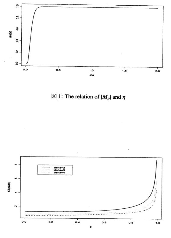
the behavior of $|M_{p}|$ when $\eta<2$ to check the effect

of non-Gaussianity. Figure 1 shows the relation of $\eta$ and $|M_{p}|$

.

Except for the region

closeto$0$,themagnitudeof_{$|M_{p}|$}

is

approximately 1,

so we

can

see

that theeffectof

non-Gaussianity is

very

small. Finally

we

see

themagnimde of$K(b,\delta)$

.

Figures2 showsthat

the relation of$K(b, \delta)$and $b$ with _$\delta=2,3$ and

4.

In

every case

the magnimde of

$K(b,\delta)$

becomes larger whenthevalueof$b$tendsto 1. Therefore thetestbased

on

Cressie-Read

power-divergence method works well for the

near

unitroot

process.

References

[1] Anderson, T. W. (1977). Estimation for autoregressive moving

average

models in

the timeandfrequency domains.Ann. Statist. 5,

842-865.

[2] Baggerly, K. A. (1998). _{Empirical likelihood}

as a

_{goodness-of-fit}

_measure.

Biometrika.85,

535-547.

[31 BRILLINGER, D. R. $(2(n1)$

.

_Time _Series: _Data_Analysis_{and Theory, expanded ed.}

Holden-Day, San Francisco.

[41 _Brockwell _P. _J. _and_Davis. _{R. A} _(1991). _Time _Series: _{Theory and}_Methods, _second

ed. Springer-Verlag.

[5] Chen, S. X. (1993). On the

accuracy

ofempiricallikelihood confidence regions for

linear regression model. Ann.Inst.Statist. Math. 45,

621-637.

[6] Chen, S. X. (1994). $Emp\ddot{m}cal$ likelihood confidence intervals for linear regression

coefficients.J. multivariate Anal. 49, 24-40.

[7] Keenan, D. M. (1987). Limiting Behavior of Functionals of Higher-Order Sample

Cumulant Spectra. Ann.Statist. 15, 134-151.

[8] Kitamura, Y. (1997). _Empirical _likelihood _methods _{with weekly dependent}

pro-cesses.

Ann. Statist. 25,

2084-2102.

[9] Monti,A.C.(1997).$Emp\ddot{m}cal$likelihoodconfidence regionsin time series models.

Biometrika. 84, 395A05.

[10] Owen, A. B. (1988). $Emp\ddot{m}cal$ likelihood ratio confidence intervals for

a

single

(15)

[11] Owen, A. B. (1990). Empirical likelihood ratio confidence regions. Ann. Statist.

18,

90-120.

[12] Owen,A.B.(1991).$Emp\ddot{m}callikelih\infty d$forlinearmodels. Ann. Statist. 19,

1725-1747.

[13] Qin, J. (1993). Empirical likelihood in biased sample problems. Ann. Statist. 21,

1182-1196.

[14] _{Qin, J. and} Lawless, J (1994). Empmcal likelihood and general estimating

equa-tions.Ann. Statist. 22,$3(n- 325$

.

[15] _{Taniguchi, M. and}Kakizawa,Y.(2000).Asymptotic Theory

_of

Statistical

_Inference

for

Time Series. Springer-Verlag, New York.

(16)

eta

図1: Therelationof$|M_{p}|$ and$\eta$

$b$