Facing the Challenges of the New European Space of Higher Education Through Effective Use of Computer Algebra Systems as an Educational Tool (Computer Algebra Systems and Education : A Research about Effective Use of CAS in Mathematics Education)

(1)

Facing the Challenges

of the

New European

Space

of Higher Education Through

Effective

Use

of

Computer Algebra Systems

as

an

Educational Tool

Andr\’es

Iglesias

Department

_of

Applied Mathematics and

Comp.

Sciences

University

_of

Cantabria,

Avda.

de los

Castros

s/n, E-39005,

Santander, Spain

iglesias@unican.es

http://personales.unican.es/iglesias

Abstract

Academic institutions of most European countries are now in the midst of the

process of overall convergence of studies at university level, the so-called European

Space

_of

HigherEducation. This process, bom from Bologna’s declaration, implies

a dramatic change in our way of teaching and learning. This change is specially

challenging in very difficult subjects such as Mathematics and other scientific dis-ciplines, which typically suffer from high failure rates. It’s author’s opinion that

Computer Algebra Systems are very powerful tools (arguably the best ones) to

face the challenges of this new approach to Higher Education. To support such

claims, some examples of Mathematica packages developed by the author during

the last few years for teaching different subjects in scientific degrees (according

to the principles and regulations ofthe European Space of Higher Education) are

briefly described.

1 Introduction

Since its signature in 1999, Bologna’s Declaration has epitomized the much-needed,

largely-demanded process of changes umdertaken in most European countries in order

to reform their Higher Education system. This agreement is not only designed for

new

curricula and academic regulations; it also accounts for

a new

approach to teaching and

learning (in author’s opinion, the most important issue of this process). This challenge

is specially important in very difficult subjects such

as

Mathematics and other scientific

disciplines, which typically suffer from high failure rates. Several academic reports have

pointed out the difficulties

our

students face when studying (and suffering) mathematical

subjects. Students and professors at university often cite

lack

of preparation from high

(2)

Right or not, the truth is Mathematics is very much practice-based.

Students

may

get

a

concept _{in the classroom, but} they will certainly lose it if not

reinforced

by

home-work. For doing so, _{students need} to be provided with good supporting materials

so

that they

can

effectively leamby themselves. High-quality, helpful educationalmaterials

allow underachievingstudents catching up on belated

as

signments and get extra time for

successful

backtracking.

It is _{at this point where Computer Algebra Systems (CAS}

on-wards)

can

reallypave _{the way, making the most with less. In author’s opinion,}

_CAS

_are

very powerful tools (arguably the best ones) to face the challenges ofthis

new

approach

to Higher Education. This paper aims at supporting such claims by presenting some

examples of Mathematica packages developed by the author during thelast few years for

teaching different subjects in scientific degrees according to the principles and regulations

of the European Space of Higher

Education.

2 _{Some Illustrative}

_Examples

2.1 Example 1:

Binary Distillation

Column

This section is about a

Mathematica

program for distillation column design described originally in [7]. This example is intended _{for students of Chemical Engineering}

de-gree who

can use

a CAS

as

a

useful tool for their symbolic/numerical computations and

graphicaloutput. For the sake of simplicity, weconsider thecaseofcontinuousdistillation

columms for binary mixtures. However,

our

approach is very general as it

can

be applied

to any other kind of distillation columns by simply replacing

our

assumptions by those

ofeach specific

case.

In this example,

we

assume

that the

colunms are

designed through

McCabe-Thiele’s

procedure [11, 12]. This is a graphical method which

determines

the number of stages required for the

desired

degree of separatIon and the

location

of the feed tray

as functions

of

some

parameters of the problem. The program isgeneral enough

to analyze

a

number of different mixtures under different conditions

as

well

as

the role

of many relevant parameters _{of this process. To this purpose,}

_an

_adequate _combination

of symbolic _{and numerical} _{calculations is achieved. From} _{these calculations, both}

nu-merical and grapluical outputs

are

obtained. In fact, the graphical output is actually

a

Mathematica

movie of

McCabe-Thiele’s

diagram.

The method has beenimplemented as a Mathematicapackage, called MTBDC.$m$, where

this acronym _{stands for McCabe- Riele Binary} _{Mstillation Column.} _{This section}

de-scribes

one

example of application of this program to

a

equimolar $(i.e. x_{f}=0.5)$ _binary

mixture whose relative volatility is $\alpha=4$

.

Our

target is to design

a

distillation column that obtains

a

destillate with 85 % of purity $(i.e. x_{d}=0.85)$ _and _bottoms _with _{5 % of}

purity $(i.e. x_{b}=0.05)$

.

The first _comand_Reflux_[xd,_xf

$l$alpha] determines three values:

the reflux, and the liquid and vapor compositions of the

more

volatile component:

In[1] $:=$ Needs$[^{1t}MCBDC$‘$||]$

In[2] $:=$ Reflux[0.85,0.5,4]

Out[2] $:=\{1.75,0.2,0.5\}$

Then, _{the command OperatingLines} [xd,_{xf, alpha]} _is _applied _{to the calculation of}

the operating _{lines of the rectification} _section _{and the} _{stripping section,} _shown _{in Fig.}

(3)

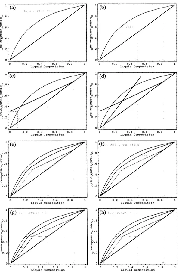
Figure 1: McCabe-Thiele’s method forbinarydistillationcolumn design: $(a)-(h)$ different

(4)

Figure 2:

McCabe-Thiele’s

method for

an

equimolar heptane-octane mixture with $x_{d}=$

0.98, $x_{f}=0.5,$ $x_{b}=0.05$ and $\alpha=2.17$: (left) _{$E_{f}=1$}; (right) _{$E_{f}=0.65$}

.

trays of the column

as

well

as

the location of the feed tray. To this end,

we

define the

MTPlot command, which accepts five different arguments, namely, $x_{d},$ $x_{f},$ $x_{b},$ $\alpha$ and the

efficiency $E_{f}$

.

For example, MTPlot [0.85,0.5,0.05,4,0.6] returns a sequence of 49

frames corresponding to the different steps of McCabe-Thiele’s method. Eight of these

frames

are

displayed in Figure 1.

One

of the most remarkable Mathematica features in this work is the possibility to

generate $Q\dot{m}ckTime^{TM}$ movies. For example, _the_{different images} _in _Figure ₁ _correspond

to eight frames of

a

QuickTime movie that reproduces _{McCabe-Thiele’s method} in a

graphical way. The movie is automatically generated from the MTPlot command.

Dif-ferent values of its arguments

are

associated with different initial mixtures and$/or$ final

products. This option is specially valuable for educational and training purposes,

as

we

can

obtain

a

virtually unlimited set of distillation columns in a fast and simple way.

McCabe-Thiele’s

method does not allow us to determine all relevant distillation

col-umn

parameters _and thus,

some

additional equations must also be considered. The

discussionis beyond the scope of this paper and will not be included here. At this time it

is enough to say that _{a number of different Mathematica commands incorporating} _these

additional

equations have been implemented in the MTBDC.$m$ package. For example, if

we

start with

an

equimolar_{mixture of heptane-octane with} _a_{relative volatility} $\alpha=2.17$ and

efficiency $E_{f}=1$ and

we

wish to obtain

a

destillate with 98 % of heptme and bottoms

with only

a

5% of heptane, the column parameters

can

be determined

as:

In[3] :$r$ ColumnParameters

$[0.98,0.05,0.5,2.17,1]$

$Out[3J:=Number$

_of

_trays _$=14$ _(rebolier _included)

Number

_of

Feed $tray=9$

Column height $=8.4$ meters

Distance

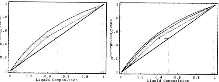
between trays $=0.6$ meters

Figure 2 shows the

McCabe-Thiele’s

diagram of the columnfor totalefficiency $E_{f}=1$

(left) and when the efficiency of the process is only a 65

%,

that is $E_{f}=0.65$ (right).

In the

first

case, the

column

has only 14 trays and its height is

8.4

meters, while in the second

case

the

number of trays increases up to

22

and the column height is

now

13.2

meters.

(5)

2.2 Example 2:

Solving

Inequalities

Solving inequalities is

a

very important topic in Mathematics, with outstanding

applica-tionsinmany

areas

oftheoretical and applied science. Inequalitiesplayakey role because

many problems cannot be completely and accurately described by using only equalities.

However, since there is not

a

general methodolody for solving inequalities, their

sym-bolic computation is still a challenging problem in computational algebra. Depending on

the kind of functions involved, there

are

many “specialized” methods such

as

cylindrical

algebraic decomposition, Gr\"oebner basis, quantifier elimination, etc. [1, 6, 8, 13].

This section

uses a

nonstandard Mathematica package [9], InequationPlot, for

dis-playing the two-dimensional solution sets of several inequalities. In particular, it extends Mathematica’s capabilities by providing graphical solutions to many inequalities (such

as

those involving trigonometric, exponential and logarithmmic functions) that cannot be

solved by using the standard Mathematica commands and packages [14, 15]. The package

also deals with inequalities involving complex variables by displaying the corresponding

solutions on the complex plane.

Inequalities involving trigonometric functions cannot be solved by standard

Mathe-matica commands. For example, let

us

try to display the solution sets of each of the

inequalities

$sin(x+y)> \frac{1}{2}$ (1)

and

$sin(2x)+cos(3y)<1$ (2)

on

the set $[$-8, $8]\cross[-8,8]$ by using the standard Mathematica commands. In this case,

we

must

use

the command InequalityPlot of the Mathematicapackage:

In[41 $:=<<Graphi$cs‘ InequalityGraphics

Unfortunately, since the regiondefined by inequality (1)

on

the prescribed domain cannot

be broken down into cylinders, Mathematica fails to give the solution:

In[5] _{$:=InequalityPlot$}$[$Sin

$[x+y]>1/2,$

$\{x,$$-8,8\},$$\{y,$_$-8,8\}]$

Out[5]: $=InequalityPlot:$ : region:

The region

_defined

by $sin(x+y)>1/2\wedge-8<=x<=8\wedge-8<=y<=8$ could not be

broken down into cylinders.

On

the contrary, the previous inequalities

can

be solved by loading

our

package:

In[6] $:=<<$InequationPlot‘

which includes the command

Inequat$i$onPlot [ineqs, $\{x$,xmin,

xmax},

$\{y$,ymin,

ymax},

opts]

for displaying the two-dimensional region of the set of points satisfying the inequalities

ineqs of real numbers inside the square [xmin,xmax] $\cross[ymin$,ymax$]$. For example,

inequalities (1)$-(2)$

can

be solved

as

follows:

In[7] _{$:=InequationPlot$} [$*,$_{$\{x,-8,8\},$}$\{y,-8,8\}$,_AspectRatio-$>Automat$ ic]& /@

$\{Sin[x+y]>1/2$,Sin$[$2 $x]+Cos[3y]<1\}$

(6)

$\infty\inftyarrow$ $\sim\lrcorner-$ $\}-$ $-$ $-$ $l$ $-$ $(\sim$

$\epsilon\}- \mathfrak{l}$ $-$ $\sim$ $-$. $-\overline{\cdot\prime\epsilon}-\backslash \overline{\epsilon}_{\vee}---1$ . 1 – —-$[$ $arrow$ $\sim$ $1$ $\}$ $($ $r\sim$ $\epsilon|$ $r\backslash$ $\nearrow\backslash$ $r\cdot-\backslash$ $’rightarrow$

Figure 3: Some examples of inequality solutions

on

the square [-8, 8] $\cross[-8,8]$: (left)

$sin(x+y)> \frac{1}{2}$; (right) $sin(2x)+cos(3y)<1$_.

Similarly, Fig. 4 displays the solution sets of the inequalities $F(x)+F(y)=1$ and

$F(x^{2})+F(y^{2})=1$ _(where $F$stands for the floor function)

on

thesquares $[$-4,$4]\cross[-4,4]$

and [-2, 2] $\cross[-2,2]$, respectively. We would like to remark that the Mathematica

com-mand InequalityPlot does not provide any solution for these inequalities either.

Figure 4: Some examples of inequality solutions: (left)

_floor

$(x)+floor(y)=1$ on the

square $[$-4,$4]\cross[-4,4]$; (right)

floor

$(x^{2})+floor(y^{2})=1$

on

_{the square} $[$-2,$2]\cross[-2,2]$.

The_{previous command, InequationPlot,}

_can

_be_{generalized to inequalities involving}

complex numbers. The

new

command

ComplexInequationPlot [ineqs, $\{z$,

{Rezmin, Rezmax},

{Imzmin,

Imzmax}},

opts]

displays the solution sets of the inequalities ineqs of complex numbers inside the square

(7)

functions appearing within the inequalities need to be real-valued functions ofacomplex argument, $e.g$

.

$Abs,$ $Re$ and $Im$. For example:

In[8] _{$:=ComplexInequationPlot$} [$\#,$$\{z,$$\{-2,3\},$$\{-3,3\}\}$,AspectRatio-$>$Automatic]& /@ $\{1<Abs[z^{rightarrow}2-z+1]<4,1<Abs[z^{-}2-2z]/$Abs$[z^{\sim}2+3]$_く₄$\}$

$Out[ 8\int:=See$ Figure 5

Figure 5: Some examples of inequality solutions for $z=a+b\in \mathbb{C}$ such that $a\in[-2,3]$

and $b\in[-3,3]$: (left) $1<||z^{2}-z+1||<4$; (right) $1< \frac{||z^{2}-2z||}{||z^{2}+3||}<4$.

$5—–\wedge^{\wedge}----\sim\sim\backslash -\sim;^{\sim}\backslash \vee\neg\sim\sim\backslash$

$1.\sim$ $\vee\backslash \backslash \backslash \backslash \backslash [_{\backslash }\backslash \backslash \backslash \backslash \backslash \llcorner$

$\sim\sim$

$–\wedge--arrow\sim$

$\sim_{s}-$

$\ell-\sim\backslash --\sim--\backslash \sim\vee^{\backslash }\cdot\backslash \wedge^{\backslash }\vee^{\backslash }\backslash \sim\backslash \backslash \backslash \sim\backslash \backslash \sim\backslash \backslash \backslash \backslash \backslash 1_{\backslash }^{\backslash }\backslash \backslash \backslash \backslash \backslash \backslash$

$\sim\sim\sim$

$\backslash f^{\mathfrak{l}}\backslash \backslash \backslash \backslash$ $\vee---arrow---\sim-$

$\backslash \backslash /\backslash$ $\backslash$

$2_{\backslash }^{-}-\backslash --\sim^{X}’/\sim\backslash \backslash \backslash \sim\backslash _{c}/’\backslash /\backslash /\backslash \backslash \backslash \backslash \backslash \backslash \backslash \backslash \backslash$

$”\nearrow’/$

ノ

$\backslash \backslash \backslash$ $\backslash /\backslash$

$0.5$ 1 1.$\lrcorner$ $2_{\lrcorner}$ 3

Figure 6: Solution sets for the inequality systems: (left) Eq. (3); (right) Eq. (4).

The last example shows how complicated the inequality systems

can

be: in

addition

(8)

compositions of these (and other) _{functions can} _{also be considered. In Figure} ₆ _the

solutions sets of the inequality systems:

$e^{y} \geq 1\wedge log(x)y\geq 1\wedge x\sqrt{y}<4\wedge x-y>\frac{1}{2}$ ₍₃₎ $log(y)\geq_{\tilde{2}}^{1}\wedge sin(x)y\geq x\wedge cos(e^{x-y})\geq 0\wedge sin(x^{2}+y^{2})>0$ ₍₄₎

on

$[1, 10]\cross[0,10]$ and $[0,3]\cross[1,5]$ respectively

are

displayed.

2.3 Example

3:

Gauss

Map

of

Surfaces

This

section

focuses

on

a

classical

topic in the field of

Differential

Geometry: the

vi-sualization of the

Gauss

map of

a

surface. Roughly speaking, the Gauss map projects

surface normals onto a unit sphere, providing a powerful visualization ofthe geometry of

a graphical object. On _{the other hand, dynamic visualization of the} _{Gauss map} _speeds

understanding

of complex surface properties. This section applies

a Mathematica

pack-age described

in [10], GaussMap, for computing and displaying the tangent and normal vector

fields

and the

Gauss

map of surfaces described symbolically in either implicit or

parametric _form. _Firstly,

_we

_load _the _package: In[9] $:=<$_くDifferentialGeometry‘GaussMap 2.3.1 Implicit _Surfaces

The ImplicitNormalField command _{calculates the normal vector field of any} _implicit

surface in the form $f(x, y, z)=0$ and retums

a

graphical output comprised of the surface

and suchanormal vectorfield. Thefirstexample is givenby theparaboloid$x^{2}+y^{2}-z=0$_:

In[10] $:=ImplicitNormalField[x^{-}2+y^{\sim}2-z,$$\{x, -2,2\},$ $\{y, -2,2\},$$\{z,$_$-1,2\}$,

Surf

ace-

$>Tme$,PlotPointsSurf

ace-

$>\{4,7\}$, VectorHead-_$>Polygon$]

$Out[10]:=See$ Figure 7

(9)

The ImplicitGaussMap command of

an

implicit surface returns the original surface and its Gauss map on the unit sphere:

In[11] $:=ImplicitGaussMap[x^{\sim}2+y^{\sim}2-z,$ $\{x,$$-2,2\},$ $\{y,$$-2,2\},$$\{z,$$-1,2\}$,

PlotPoints-$>\{4,7\}]$

Out

$[$ll$]$ $:=See$ Figure

8

Figure 8: (left) Implicit surface $x^{2}+y^{2}-z=0$; (right) its

Gauss

map. Next example calculates the normal vector field of the surface $z-x^{2}+y^{2}=0$:

In[12] $:=ImplicitNormalField[z-x^{-}2+y^{\sim}2,$$\{x, -2,2\},$ $\{y, -2,2\},$$\{z,$$-2,2\}$,

Surf

ace-

$>True$, PlotPointsSurf

ace-

$>\{4,6\}$,VectorHead-$>Polygon$ ,

PlotPointsNormalField-$>\{3,4\}]$

Out[12]:$=See$ Figure 9

Figure 9: The surface $z-x^{2}+y^{2}=0$ _and _{its vector} _{normal field.}

The Gauss map image of such a surface is obtatned

as:

In[13] $:=ImplicitGaussMap[z-x^{arrow}2+y^{arrow}2,$ $\{x,-2,2\},$$\{y, -2,2\},$$\{z,-2,2\}$,

PlotPoints-$>\{4,6\}]$

(10)

Figure

10:

(left) Implicit surface $z-x^{2}+y^{2}=0$_; _(right) _{its Gauss} _map.

A

more

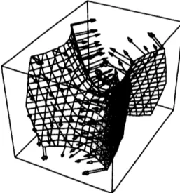
complicated example is given by the double toms surface, defined implicitly

by $(\sqrt{(\sqrt{x^{2}+y^{2}}-2)^{2}+y^{2}}-2)^{2}+z^{2}-1=0$ _{and whose} _{normal vector field is shown}

in Figure 11:

In[14] _{$:=ImplicitNormalField[$}$($Sqrt$[$(Sqrt_{$[x^{-}2+y^{\sim}2]-2$}) _{$2+y^{\sim}2]-2)^{\wedge}2+z^{\wedge}2-1$}

.

$\{x,$$-6,6\},$$\{y,-4,4\}_{*}\{z,$$-1,1\}$, Surface-$>True$, VectorHead-$>Polygon$,

PlotPointsSurf

ace-

$>\{5.5\}]$

Out$[$

14

$]$ $:=See$ Figure11

Figure 11: The double torus surface and its vector normal field.

In[15] _{$:=ImplicitGaussMap[$}$($Sqrt$[$(Sqrt_{$[x^{\wedge}2+y^{\wedge}2]-2$}) _{$2+y^{\text{へ}}2]-2)^{arrow}2+z^{rightarrow}2-1$} ,

$\{x,-6,6\},$ $\{y,-4,4\},$$\{z,-1,1\}$,Pl_{$otPoints->\{5,5\}]$}

Out[15]:$=See$ Figure 12

It is interesting to remark that,

because

the Gauss map is a continuous (in fact,

(11)

Figure 12: (left) Double torus surface; (right) its

Gauss

map.

compact sets.

Since

the double torus is compact, its image is actually the unit sphere.

Another example ofthis property is the Lam\’e surface of fourth degree $x^{4}+y^{4}+z^{4}=1$:

In[16]:$=ImplicitNormalField[x^{\sim}4+y^{arrow}4+z^{-}4-1,\{x,-1,1\},$$\{y,-1,1\},$$\{z,-1,1\}$,

Surface-$>Tme$, PlotPointsSurface-$>\{4,6\}$, VectorHead-_$>Polygon$]

Out$[$16$]:=See$ Figure 13

Figure 13: The surface $x^{4}+y^{4}+z^{4}=1$ and _its vector normal field.

Its corresponding Gauss map image

can

displayed as:

In[17] $:=ImplicitGaussMap[x^{rightarrow}4+y^{arrow}4+z^{-}4-1,$$\{x,-1,1\}$,$\{y, -1,1\}$ ,

$\{z , -1,1\}$,PlotPoints-$>\{4.6\}]$

Out$[$17$]:=See$ Figure 14

2.3.2 Parametric Surfaces

As indicated above, the package also deals with surfaces given in parametric form. In the

following example,

we

consider the Mobius strip, parameterized by

(12)

Figure 14: Lam\’e _{surface of fourth} _{degree; (right) its}

_Gauss

_map.

Figures 15 and 16 show its normal vector field and the Gauss map, respectively.

In[18]:$=$

ParametricNormalField

$[\{Cos[u]+v$

Cos$[u]$ _Sin$[u/2]$ _,

Sin$[u]+v$ _Sin$[u/2]$ _Sin$[u],v$ _Cos$[u/2]\},$$\{u,$$0,4$ Pi,Pi/10$\}$,

$\{v, -1/2,1/2,0.1\}$,Surf

ace-

$>True$, PlotPoints-$>\{50,7\}$,

SurfaceDomain-$>\{\{0,2$ Pi$\},$$\{-1/2,1/2\}\},VectorHead->Polygon$,

HeadLength-$>0.25$,HeadWidth-$>0.1$,_VectorColor-_{$>RGBColor[1,0,0]]$}

$Out[18]:=See$ Figure 15

Figure 15: The M\"obius _strip _{and its vector} _{normal field.}

In[19]:_{$=ParametricGaussMap[\{Cos[u]+v$} _Cos_$[u]$ _Sin_$[u/2]$ _{, Sin}_$[u]+$

$v$ Sin$[u/2]$ Sin$[u],$$v$ Cos$[u/2]\},$$\{u,0,4Pi\},$$\{v$,-1/2,1/2$\}$,

SurfaceDomain-$>\{\{0,2$ Pi$\},$_{$\{-1/2,1/2\}\}$},PlotPoints_{$->\{50,7\}]$}

$Out[19]:=See$ Figure16

2.4 Example 4:

Solving

Functional

Equations

In this section

we

use

the

Mathematica

package FSolve [3, 4], implemented to solve

functional

equations [2, 5].

Let’s

start loading the package:

(13)

Figure

16:

(left) M\"obius strip surface; (right) its

Gauss

map.

It includes the command: FSolve[$eqn$,

{functions}, {variables},

options] where $eqn$

denotes thefunctionalequation tobesolved,

_{functions}

isthe listofunknownfunctions,

{variables}

is the list of variables and options allows the

users

to consider different domains for the variables (see Table 1) and classes offeasible

functions

(see Table 2).

Table 1: List of all feasible domains used in the FSolve package.

(14)

Table 2:

Classes

offeasible fumctions used in the FSolve package.

$g(x)+h(y)$ where $x,$$y\in \mathbb{R}$ and $f,$$g,$$h$

are

continuous

functions

as:

In[21] $:=$ FSolve$[f[x+y]==g[x]+h[y],$$\{f$,$g,h\},$$\{x,y\}$,Domain-_$>Real$_,

Class-$>$Continuous]

Out[21] _{$:=\{f(x)arrow C(1)x+C(2)+C(3), g(x)arrow C(1)x+C(2), h(x)arrow C(1)x+C(3)\}$}

where

$C(1),$ $C(2)$

and

$C(3)$

are

arbitrary

constants. Note

_that

a

_{single equation}

_can

determine

several

unknown

functions (such

as

$f,$$g$ and $h$ in this example). Notealso that

the solution

can

depend on one or

more

arbitrary constants and$/or$ arbitrary functions: In[22] _{$:=FSolve[f[x]*Sin[y]+h[x]*g[y]==0, \{f , g,h\}, \{x,y\}]$}

$\{\{f[x]arrow 0, g[y]arrow C[0]Sin[y]+C[1]Arb[0][y], h[x]arrow 0\}$_,

Out[22]

$:= \{f[x]arrow C[1]Arb[0][x], g[y]arrow-\frac{C[1]Sin[y]}{C[0]}, h[x]arrow C[0]Arb[0][x]\}\}$

In[23] _{$:=FSolve[k[u]*1[v]==-b[u] , \{k, 1,b\}, \{u,v\}]$}

Out[23] $:=$ $\{\{k[u]arrow 0, b[u]arrow 0, l[v]arrow C[0]+C[1]*Arb[0][v]\}$,

$\{k[u]arrow C[0]*Arb[0][u],$ _{$b[u]arrow C[1]*Arb[0][u],$}_{$l[v]arrow-(C[1]/C[0])\}\}$}_,

In[24]:

_{$=FSolve[f[g[x]+h[y]]-s[r[x]+s[y]]==0,$}

_$\{f,g,h.r,$_$s\},$_$\{x,y\}$_,

Domain-$>RealPositive$ ,Class-$>Arbitrary$]

Out

$[$

24

$]$ _$:=$ _{$\{\{f[x]arrow s[\frac{x-C|2\rceil-C[3\rceil}{C[1]}],$}$g[x]arrow C[2]+C[1]r[x],$

$h[x]arrow C[3]+C[1]s[x]\}\}$

Acknowledgments

This

paper

is the printed version of

an

invited talk delivered by the author at RIMS

(Research

_Institute

_for

_Mathematical

_{Sciences) workshop}

_on

_Computer _{Algebra Systems}

andEducation; _{A Research}_about

_Effective

_Use

_of

_CAS

_in

_Mathematics

_{Education, Kyoto}

University (Japan), August $29th$

.

2008.

The author would like _to thank the _organizers

of this exciting

RIMS

workshop for their diligent work and kind invitation. Special thanks

are

owe

to

Prof. Setsuo

Takato (Toho University, Japan) for his friendship, his

great support and hospitality and for making my stay in Kyoto such a wonderful and

unforgettable experience.

It

was

indeed alovely time I will

never

forget. Doomo antgatoo

(15)

This research has been supported by the Computer Science National Program of

the Spamish Ministry of Education and Science, Project Ref.

#TIN2006-13615

and the

University of Cantabria.

References

[1] Beckenbach, E.F., Bellman, R.E.: An Introduction to Inequalities. Random House,

New York (1961).

[2] Castillo, E., Guti\’errez, J.M., Iglesias, A.: Solving

a functional

equation. The

Mathe-matica Joumal, 5(1) (1995) 82-86.

[3] Castillo, E., Iglesias, A., Cobo, A.: A package for symbolic solutions of

fmctional

equations. In: Keranen, V., Mitic, P. (Eds.): Proceedings of the First

Intema-tional Mathematica Symposium. Computational Mechanics Publications, $Southam\triangleright$

ton (England), pp. 85-92.

[4] Castillo, E., Iglesias, A.: A package for symbolic solution of real functional equations

of real variables. A equationes Mathematicae, 54 (1997) 181-198.

[5] Castillo, E., Iglesias, A., Ruiz-Cobo, R.: Functional Equations in Applied

Sciences.

Elsevier Pub., Amsterdam (2005).

[6] Caviness, B.F., Johnson, J.R.: Quantifier Elimination and Cylindrical Algebmic

De-composition. Springer-Verlag, New York (1998).

[7] Ga’lvez, A., Iglesias, A.: Binary distillation column design using Mathematica.

Lec-tures Notes in Computer Science, 2657 (2003) 848-857.

[8] Hardy, G.H., Littlewood, J.E., P\’olya, G.: Inequalities (Second Edition). Cambridge

University Press, Cambridge (1952).

[9] Ipanaqu\’e, R., Iglesias, A.: A Mathematica packagefor solving and displaying

inequal-ities.

Lectures

Notes in Computer Science,

3039

(2004)

303-310.

[10] Ipanaqu\’e, R., Iglesias, A.: A Mathematica package for computing and visualizing

the Gaussmap of surfaces. Lectures Notes in ComputerScience, 3482 (2005) 492-501.

[11] McCabe, W.L., Thiele, E.W.: Graphical design of distillation columns, Ind. Eng.

Chem., 17 (1925) 605.

[12] McCabe, W.L., Smith, J. C., Harriott, P.: Unit Operations

_of

Chemical Engineering,

Sixth Edition, McGraw-Hill, Boston (2001).

[13] McCallum, S.: Solving polynomial strict inequalities using cylindrical algebraic

de-composition. The Computer Joumal, 36(5) (1993) 432-438.

[14] Strzebonski, A.: An algorithm for systems of strong polynomial inequalities. The Mathematica Joumal, 4(4) (1994) 74-77.

[15] Strzebonski, A.: Solving algebraic inequalities. The Mathematica Joumal, 7 (2000)