The "yuima" package : an R framework for simulation and inference of stochastic differential equations (Frontiers in mathematical science through collaborations with other disciplines)

The

yuima

package:

an

R framework

for

simulation

and

inference of stochastic

differential

equations

Stefano

Maria

Iacus

Department

of

Economics,

Business

and

Statistics

University of Milan

Via

Conservatorio

7,

20124

Milan,

Italy

Abstract

The Yuima Project is an open source and collaborative effort of several mathematicians and statisticians aimed at developing the $R$

package named “yuima” for simulation and inference of stochastic dif-ferential equations.

In the yuima package stochastic differential equations can be of very abstract type, e.g. uni or multidimensional, driven by Wiener process of fractional Brownian motion with general Hurst parameter, with or without jumps specified as L\’evy noise. L\’evy processes can be specifiedvia compound Poisson description, by the specificationofthe L\’evy measure or via increments and stable laws.

The yuima package is intended to offer the basic infrastructure on

whichcomplexmodels and inferenceprocedurescanbe built on. In par-ticular, the basic set of functions includes the following: i) simulation

schemes for all types ofstochastic differential equations (Wiener, $fBm$,

L\’evy); ii) different subsampling schemes including random sampling withuserspecifiedrandom timesdistribution,spacediscretization, tick times, etc. iii) automatic asymptotic expansion for the approximation andestimationof functionals of diffusion processes with small noise via Malliavincalculus, usefulin optionpricing; iv) efficient quasi-likelihood inference for diffusion processes and model selection.

1

Introduction

The YUIMA Projectl is an open

source2

academic project aimed at

develop-ing the $R$ package named “yuima” for simulation and inference of stochastic

differential equations. The YUIMA Project is mainly developed by

mathe-maticians and statisticians who actively publish in the field of inference and simulation for stochastic differential equations. The YUIMA Project Core

Team, currently consists of the following people: A. Brouste, M. Fukasawa,

H. Hino, S.M. Iacus, K. Kamatani, H.Masuda, Y. Shimizu, M. Uchida, N. Yoshida.

The yuima package provides an object-oriented programming

environ-ment for simulation and statistical inference for stochastic processes by R.

The yuimapackage adopts the S4 system of classes and methods (Chambers,

1998).

Under this framework, the yuima package also supplies various functions

to execute simulation and statistical analysis. Both categories of procedures

may depend each other. Statistical inference often requires a simulation

tech-nique as a subroutine, and a certain simulation method needs to fix a tuning

parameter by applying a statistical methodology. It is especially the case of

stochastic processes because most of expected values involved do not admit an

explicit expression. The yuima package facilitates comprehensive, systematic

approaches to the solution.

Stochastic differential equations arecommonly usedtomodelrandom

evo-lution along continuous or practically continuous time, such

as

the random

movements of a stock price. Theory ofstatistical inference for stochastic dif-ferential equations already has afairly long history, more than three decades,

but it is still developing quickly new methodologies and expanding the

area.

The formulas produced by the theory are usually very sophisticated, which

makes it difficult for standard users not necessarily familiar with this field to

enjoy utilities. Forexample, the asymptotic expansion method for computing

option prices (i.e., expectation of an irregular functional of a stochastic

pro-cess) providesprecise approximation valuesinstantaneously, taking advantage

of the analytic approach, but the formula has along expression likemorethan

one page!

Theyuimapackage delivers up-to-datemethodsas apackageontothedesk

of the userworking with simulation and/or statistics forstochastic differential

equations.

Sampled data from a continuous-time process features the time stamps

as

well as the positions of the object. It is requiring a new theory of estimation. lThe Project has been funded upto2010 by the JapanScienceTechnology (JST) Basic

Research Programs PRESTO, Grants-in-Aidfor Scientific Research No. 19340021.

2All codein the yuima packageis subject to the GNU General Public License, Version

The yuima framework can apply multi-dimensional time stamps of tick data and provides diverse functions handling such kind data to support statistical analysis.

Although we assume that the reader of this paper has a basic knowledge

ofthe $R$ language, most of theexamples are easy to be understoodby anyone.

2

The

yuima

package

The package yuimna depends on some other packages, like zoo, which can be

installed separately. The package zoo is used intemally to store time series

data. This dependence may change in the future adopting a more flexible class for internal storage of time series.

2.1

How

to obtain the package

The yuima package is hosted on R-Forge and the web page of the Project is

http:$//r$_{-forge. r-project.org/projects/yuima.} The R-Forge page

con-tains the latest development version, andstable version ofthe package as also available through CRAN. Development versions of the package are not

sup-posed to be stable or functional, thus the occasional user should consider to

install thestableversion first. The packagecan beinstalIed$hom$ R-Forge using

install.packages (“yuima”,repos $=”$_{http $://R$-Forge.R-proj ect. org”)}

and for the CRAN version, via install.packages(“yuima”).

2.2

The

main object and classes

Before discussing the methods for simulation and inference for stochastic

pro-cesses solutions to stochastic differential equations, here we discuss the main

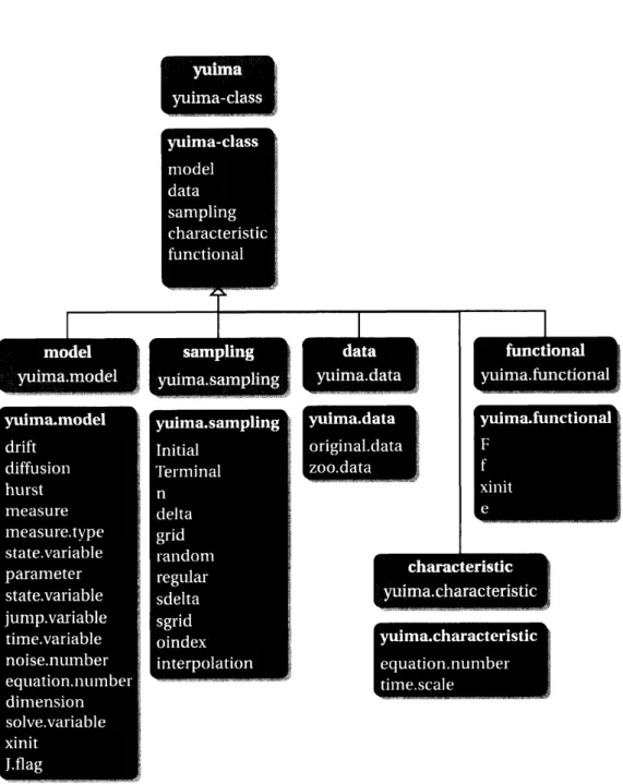
classes in the package. As mentioned there are different classes of object de-fined in the yuima package and the main class is called the yuima-class and

it is composed of several slots. Figure 1 represents the different classes and

their slots. The different slots do not need to be all present at the

same

time. For example, in case one wants to simulatea stochastic process, only the slots

model and sampling should be present, while the slot data will be filled by the simulator. We now discuss in details the different object separately.

2.3

The

yuima.model

class

In yuima three main classes of stochastic differential equations can be easily specified. All multidimensional and eventually as parametric models.

$\bullet$ diffusions $dX_{t}=a(t, X_{t})dt+b(t, X_{t})dW_{t}$, where $W_{t}$ is astandard

$\bullet$ fractional Gaussian noise, with $H$ the Hurst parameter

$dX_{t}=a(t, X_{t})dt+b(t, X_{t})dW_{t}^{H}$;

$\bullet$ diffusions with jumps and L\’evy processes solution to

$dX_{t}=a(X_{t})dt+b(X_{t})dW_{t}+\int_{|z|>1}c(X_{t-}, z)\mu(dt, dz)$

$+ \int_{0<|z|\leq 1}c(X_{t-}, z)\{\mu(dt, dz)-\nu(dz)dt\}$.

The yuima. model class contains informations about the stochastic differ-entialequation ofinterest. The constructor setModel is used to give a

mathe-matical description ofthe stochastic differentialequation. All functions inthe

package are assumed to get

as

much information

as

possible from the model instead of replicating the

same

code everywhere. If there

are

missing pieces of information, we may change or extend the description of the model. An object of yuima. model contains several slots listed below. To see inside

its structure, we use the $R$ command str.

$\bullet$ drift is an $R$ expression which contains the drift specification.

$\bullet$ diffusionis itself alistof 1slot which describes thediffusion coefficient

relative to first noise.

$\bullet$ parameter which is a short name for “parameters” which is a list of

objects.

$\bullet$ all contains the

names

of all the parameters found in the diffusion and

drift coefficient.

$\bullet$ common contains the names of the parameters in common between

the.

drift and diffusion coefficients.

$\bullet$ diffusion contains the parameters belonging to the diffusion

coeffi-cient.

$\bullet$ drift contains the parameters belonging to the drift coefficient.

$\bullet$ solve. variable contains avector of variable names, each element

cor-responds to the name of the solution variable (left-hand-side) of each

$\bullet$ state. variable and time.variable, by default, are assumed to be

$x$

and $t$ but the user can freely choose them. The yuima.model function

assumes that the user either usedefault names for state. variable and

time. variable variables or specify his own

names.

All the rest of the

symbols are considered parameters and distributed accordingly in the

parameter slot.

$\bullet$ noise. number indicates the number of sources of noise.

$\bullet$ equation.number represents the number of equations, i.e. the number

of one dimensional stochastic differential equations.

$\bullet$ dimension reports the dimensions ofthe parameter space. It is a list of

the same length of parameter with the same names.

In order to show how general is the approach in the yuima package we

present some examples.

2.3.1 Diffusion processes

Assume that we want to describe the following stochasticdifferential equation

$dX_{t}=-3X_{t}dt+\frac{1}{1+X_{t}^{2}}dW_{t}$

This is done in yuima specifying the drift and diffusion coefficients as plain

mathematical expressions

$R>modl$ $<-setMo$del(drift $=$ $-3*x’$‘,

$+$ _$di$ffusion $=$ $|l/(1+x^{\sim}2)$“$)$

At this point, the package fills the proper slots of the yuima object

$R>$ str(modl)

Formal class ’yuima.model‘ [package “yuima“] with 16 slots

$Q$ drift : expression$((-3*x))$

..@ diffusion :List of 1

. . ..$: expression$(l/(l +x^{-}2))$

@ hurst : num 0.5

..@jump. coeff : expression$()$

. .$Q$ measure : list_$()$ ..6 measure.type : chr(0)

. .@ parameter : Formal class model. parameter$t$

[package “_{yuima“] with 6 slots}

.,@ all : chr(0) .. . . .. $\emptyset$ common : chr(0) .. . . . .$Q$ diffusion: chr(0) ..@ drift : chr(0) . . . . .. ..@ jump : chr(0) . .$Q$ measure : chr(0) .. $\Phi$ state.variable: chr _$x”$ ..$Q$ jump.variable : chr(0) ..$Q$ time.variable : chr $|t^{\prime 1}$

..0 equation.number: int 1

$Q$ dimension : int [1:610 $00000$

$Q$ solve.variable : chr $x”$

..$Q$ xinit : num $0$ ..$Q$ J.flag : logi FALSE

And it is possible to

see

that the jump coefficient is void and the Hurst

parameter is set to 0.5, because this corresponds to the standard Brownian motion. Now, with modl in hands, it is very easy to simulate a trajectory of the process as follows

$R>$ set.seed(123)

$R>X<$-simulate(modl) $R>plot$(X)

0.0 02 0.4 06 0.8 1.0

$t$

The simulate function fills in addition the two slots data and sampling of

the yuima object.

$R>$ str(X, vec. 1 en $=2$)

Formal class yuima‘ [package $|yuima^{1\mathfrak{l}}$] with 5 slots

$Q$ data :Formal class ‘yuima.data‘ [package “yuima”] with 2 slots ..$Q$ original.data; ts [1:101. 1] $0$ -0.056 .. .

..

. . .. . . .$.-$ attr($*,$ dimames)$\cdot List$ of 2

.. . . ..$: NULL .. .. . . .. . . ..$: chr “Series 1“ .. . . .. .$.-$ attr$(*, tsp)-$ num [1:3] 01100 $Q$ zoo.data :List of 1 .

.

..$ Series 1:$g\ddot{Y}zooregil2$ series from $0$ to 1

..

Data; num [1; 101] $0$ -0.056 ...

Index: num [1:101] $0$ 0.010.02 0.03 0.04 . ..

Frequency; 100

..$Q$ model :Formal class ’yuima. model‘ [package “yuima”] with 16 slots $Q$ drift : expression$((-3*x))$ .. . . . . $Q$ diffusion :List of 1 .

.

.. .. ..$: expression$(l/(l +x2))$ $Q$ hurst : num 0.5 ..

.. .. $Q$ jump. coeff : expression$()$

$Q$ measure : list$()$

. .

. . . .$Q$ measure.type : chr(0)

..$Q$ parameter : Formal class ’model.paramoter’ [package ”yuima”] with 6 slots .. .. .. .. .. . .$Q$ all : chr(0) . . . . .. . . $\Phi$ common : chr(0)

. .

. . .. ., . .$Q$ diffusion: chr(0) . . . .. . .$Q$ drift : chr(0) . . .. . . .. $Q$ jump : chr(0)

. . . .. . .$Q$ measure ; chr(0) .. . . $\emptyset$ state.variable: chr )_$t|x$’ . . $Q$ jump.variable : chr(0) . . . . ..6 $t$ime.variable ; chr ${}^{t}t’$ . . . . ..@ noise.number : num 1 . . . . ..@equation.number: int 1 .. . . $Q$ dimension : int [1;6] $00000$ ... $Q$ solve.variable ; chr $x^{I1}$ . . . . .. ..@ xinit : num $0$ . . $Q$ J.flag ; logi FALSE

$Q$ sampling :Formal class yuima.sampling‘ [package ”yuima“] with 11 slots

$Q$ Initial : num $0$ ..

. . . . $\Phi$ Terminal : num 1

. . . . $Qn$ ; _num 100

. . . .$Q$ delta : num 0.01 . . . . $Q$ grid :List of 1

..$: num [1:101] $0$ 0.010.02 0.03 0.04 . . .

..

. . . . ..@ random ; _{logi FALSE}

.

.

. .$\emptyset$ regular : logi TRUE

. . . . ..@sdelta : num(0)

..@ sgrid : num(0)

. .

. . . . $Q$ oindex : num(0) . . $Q$ interpolation: chr “pt’t

$Q$ characteristic:Formal class $|yuima.characteristic$’ [package ”yuima“] with 2 slots .. $\mathfrak{g}$ equation.number; int 1

..@ time.scale : num 1

. .

. .$Q$ functional :Formal class lyuima.functional‘ [package “yuima”] with 4 slots .,$QF$ _{: NULL}

. .

.. . . ..6 $f$ $:1ist()$

. . .. $\emptyset$ xinit: num(0)

..Qe _: num(0)

..

2.3.2 Parametric models

When a parametric model like

$dX_{t}=-\theta X_{t}dt+\frac{1}{1+X_{t}^{\gamma}}dW_{t}$

is specified, yuima attempts to distinguish the parameters’ names from the

ones of the state and time variables

$R>mod2$ $<-setModel(drift=$ $”-theta*x”$,

$+$ $dif$fusion $=$ “$1/(1+x^{-}gamma)$ “$)$

$R\succ$ str(mod2)

Formal class yuima.modelt [package ‘yuima“] with 16 slots $\Phi$ drift : expression((-theta $*x)$ )

.

.$Q$ diffusion :List of 1 .. ..$: expression(l/(l $+x^{-}$gamma$)$)

.

.$G$ hurst : num 0.5 . .$Q$ jump.coeff : expression$()$ . .$Q$ measure : list$()$ . .$Q$ measure.type ; chr(0)

. .$Q$ parameter :Formal class model.parameter$|$

[package ”yuima”] with 6 slots

..$\Phi$ all ; chr [1:2] $1\dagger$

thet$a^{11}$ “gamma”

..

..@ common : chr(0)

..

. . . . ..$Q$ diffusion; chr ”gamma“

$\Phi$ drift : chr 1ltheta”

. . . . $Q$ jump : chr(0) . .$Q$ measure : chr(0) . . $Q$ state.variable: chr $x^{1\prime}$ ..9 jump.variable : chr(0) . .$Q$ time.variable : chr $t$“ $Q$ noise.number : num 1 ..$Q$ equation.number: int 1 $Q$ dimension : int [1:6] 2 0110 $0$ . .$Q$ solve. variable : chr _$x”$ . .$Q$ xinit : num $0$ $Q$ J.flag ; logi FALSE

In order to simulate the parametric model it is necessary to specify the values

of the parameters as the next code shows

$R>set.$seed(123)

$R>X<$-simul ate(mod2, _{true.par$am=list$}(theta $=1$,

$+$ gamma $=3$)$)$

$R>plot$(X)

0.0 02 04 06 08 10

$t$

2.3.3 Multidimensional processes

Next is an example with two stochastic differential equations driven by three

independent Brownian motions

$dX_{t}^{1}=-3X_{t}^{1}dt+dW_{t}^{1}+X_{t}^{2}dW_{t}^{3}$

$dX_{t}^{2}=-(X_{t}^{1}+2X_{t}^{2})dt+X_{t}^{1}dW_{t}^{1}+3dW_{t}^{2}$

but this has to be organized into matrix form

$(dX_{t}^{2}dX_{t}^{1})=(\begin{array}{l}-3X_{t}^{l}--X_{t}^{1}2X_{t}^{2}\end{array})dt+\{\begin{array}{lll}1 0 X_{t}^{2}X_{t}^{1} 3 0\end{array}\}(dW_{t}^{3}dW_{t}^{2}dW_{t}^{1})$

$R>sol<-c(^{\prime l}x1’’$, “x2“$)$

$R>$ a _$<-c$$(”-3*xl ”, ”-xl-2*x2”)$

$R>b<$-matrix$(c(^{ll}l$ ”, $xl$”, $0^{l\prime}$, $3^{\prime l}$,

$+$ $x2^{\iota\prime}$, _$|0’’),$ $2,3)$

$R>mod3$ $<$-setModel(dri$ft=a,$ _$di$ffusion _$=b$, $+$ $solve$

.

vari$able=sol$)

Again, this model can be easily simulated

$R>$ set.seed(123)

$R>X<-simul$ate(mod3)

$R>plot$ (X, plot.type $=$ “si_$ngle^{t},$ $lty=1:2$)

00 02 04 0.6 08 10

1

But it is also possible to specify more complex models like the following

$\{\begin{array}{l}dX_{t}^{1}=X_{t}^{2}|X_{t}^{1}|^{2/3}dW_{t}^{1},dX_{t}^{2}=g(t)dX_{t}^{3}, ,dX_{t}^{3}=X_{t}^{3}(\mu dt+\sigma(\rho dW_{t}^{1}+\sqrt{1-\rho^{2}}dW_{t}^{2}))\end{array}$

where $g(t)=0.4+(0.1+0.2t)e^{-2t}$.

2.3.4 Fractional Gaussian noise

In order tospecify a stochastic differentialequation driven byfractional

Gaus-sian noise it is necessary to specify the value of the Hurst parameter. For example, ifwe want to specify the following model

$dY_{t}=3Y_{t}dt+dW_{t}^{H}$

we proceed as follows

$R>mo$_d4 $<-s$_etModel$(drift=$ “_{$3*y^{l\prime}$},

$+$ diffusion $=1$, hurst $=0.3$,

$+$ solve._{$var=|y\uparrow’)$} $R>set.$seed(123)

$R>X<$-simul ate(mod4, sampling $=$ setSampli$ng(n=1000)$)

00 02 0.4 06 0.8 10

$t$

In this case, the appropriate slot is now filled

$R\succ str(mod4)$

Formal class yuima.model‘ _{[package “yuima”] with 16 slots}

..$Q$ drift ; expression $((3 *y))$ . .$Q$ diffusion :List of 1

. . ..$: expression(l)

. .$Q$ hurst : num 0.3 ..$Q$ jump. coeff : expression$()$

. .$\emptyset$ measure : list$()$

. .$Q$ measure.type : chr(0)

. .$Q$ parameter ;Formal class ‘model.parametert [package “yuima”]

with 6 slots $Q$ all ; chr(0) . . . . .. $Q$ common : chr(0) .. .. ..0 diffusion: chr(0) . . . . $Q$ drift : chr(0) .. $Q$ jump : chr(0) . .$Q$ measure ; chr(0) . . ..$Q$ state.variable: chr $x”$ $Q$ jump.variable : chr(0) $Q$ time. variable : chr $t^{\prime\iota}$

$Q$ noise.number : num 1 $Q$ equation.number: int 1 ..$Q$ dimension ; int [1:6] $000000$ $Q$ solve.variable; chr $|\prime y’’$ $Q$ xinit : num $0$

$Q$ J.flag _; logi FALSE

2.3.5 L\’evy processes

Jump processes

can

be specified in different ways in mathematics and hence

in yuima package. Let $Z_{t}$ be a Compound Poisson Process (i.e. jumps follow

some distribution, like the Gaussian law). Then it is possible to consider the

following SDE which involves jumps

$dX_{t}=a(X_{t})dt+b(X_{t})dW_{t}+dZ_{t}$

In the next example we consider a compound Poisson process with intensity

$\lambda=10$ with Gaussian jumps. This model can be specified in _setModel

us-ing the argument measure.type$=t\dagger$

CP$11$ A

simple Ornstein-Uhlembeck process

with Gaussianjumps

$dX_{t}=-\theta X_{t}dt+$ad$W_{t}+Z_{t}$

$R>mod5$ $<-$ se$tModel(drift=c$$(”-theta*x^{t\prime})$,

$+$ diffusion $=$ sigm$a^{l1}$, jump.coeff $=$ “1 “,

$+$ measure $=list$(intensity $=\prime\prime 10$“,

$+$ $df=list$(”dnorm(

$z,$ $0$, I) “)$)$,

$+$

measure.

$type=$ “_$CP$“, $solve$

.

vari_{$able=\iota_{X^{l\dagger)}}$} $R>set.$seed(123)

$R>X<$-simul ate(mod5, _tru

_$e.p=list$

(theta $=1$,

$+$ _$si$gma $=3$), _$s$ampl$ing=s$etSampl$ing(n=1000))$

$R>plot$(X)

0.0 02 0.4 0.6 0.8 10

$t$

Another possibility is to specify the L\’evy measure. Without going into

too much details, here is an example of specification of a simple Ornstein-Uhlembeck process with IG (Inverse Gaussian) L\’evy measure

$dX_{t}=-xdt+dZ_{t}$

$R>mod6$ $<$-setModel $(drift=$ $”-x^{\prime 1}$, $+$ xinit $=1,$ _$j$ump. coeff $=$ “1“,

$+$ measure.$type=$ “code“, measure $=list$_{$(df=||r\mathcal{I}G(z, 1,0.1) "))$}

$R>set.$seed(I23)

$R>X<$-simul ate(mod6, sampling $=$ setSampl_$ing$(Terminal $=10$,

$+$ $n=1$0000$))$

$R>plot$(X)

$0$ 2 ₄ 6 8 40

2.3.6 Generic models

In general, the yuima package allows to specify a large family of models solutions to

$dX_{t}=a(X_{t})dt+b(X_{t})dW_{t}+c(X_{t})dZ_{t}$

using the following interface

$R>$ setModel $(drift,$ $di$ffusion, hurst $=0.5$,

$+$ jump. coeff, measure, measure.type,

$+$ _$st$a_$te$

.

varia$ble=$ _$x”$, jump. varia$ble=\iota\prime z^{l\prime}$,

$+$ $time$

.

varia$ble=$ $|t$“, solve.varia$ble$,

$+$ _$xi$nit)

The yuima package implements many multivariate Random Numbers Gener-ators (RNG) which are needed to simulate L\’evy paths including $rIG$ (Inverse

Gaussian), $rNIG$ (Normal Inverse Gaussian), rbgamma (Bilateral Gamma),

rngamma (Gamma) and rstabIe (Stable Laws). Other user-defined RNG can

be used freely.

3

Asymptotic expansion

The yuima package can handle asymptotic expansion of functionals of d-dimensional diffusion process

$dX_{t}^{\epsilon}=a(X_{t}^{\epsilon}, \epsilon)dt+b(X_{t}^{\epsilon}, \epsilon)dW_{t}$ , $\epsilon\in(0,1]$

with $W_{t}$ and r-dimensional Wiener process, i.e. $W_{t}=(W_{t}^{1}, \ldots, W_{t}^{r})$. The

functional is expressed in the following abstract form

$F^{\epsilon}(X_{t}^{\epsilon})= \sum_{\alpha=0}^{r}\int_{0}^{T}f_{\alpha}(X_{t}^{\epsilon}, d)dW_{t}^{\alpha}+F(X_{t}^{\epsilon}, \epsilon)$, $W_{t}^{0}=t$

A typical example of application is the case of Asian option pricing. For

example, in the Black

&

Scholes model

$dX_{t}^{\epsilon}=\mu X_{t}^{\epsilon}dt+\epsilon X_{t}^{\epsilon}dW_{t}$

the price of the option is of the form

$E\{\max(\frac{1}{T}\int_{0}^{T}X_{t}^{\epsilon}dt-K,$ $0)\}$

.

Thus the functional of interest is

with

$f_{0}(x, \epsilon)=\frac{x}{T}$, $f_{1}(x, \epsilon)=0$, $F(x, \epsilon)=0$

in

$F^{\in}(X_{t}^{\epsilon})= \sum_{\alpha=0}^{r}\int_{0}^{T}f_{\alpha}(X_{t}^{\epsilon}, d)dW_{t}^{\alpha}+F(X_{t}^{\epsilon}, \epsilon)$

So, the call option price requires the composition of a smooth functional

$F^{\epsilon}(X_{t}^{\epsilon})= \frac{1}{T}\int^{T}X_{t}^{\epsilon}dt$, $r=1$

with the irregular function

$\max(x-K, 0)$

Monte Carlo methods require a huge number of simulations to get the desired

accuracy of the calculation of theprice, while asymptotic expansionof$F^{\epsilon}$

pro-vides very accurate approximations. The yuima package provides functions

to construct thefunctional $F^{\epsilon}$, and automatic asymptotic expansionbased on

Malliavin calculus starting from a yuima object. Next is an example

$R>diff$

.

matrix $<$-matrix$(c(^{ll}x*e^{\prime\downarrow})$, $+$ 1, 1)

$R>$ model $<-setModel$_(drift $=c(\prime\prime x’’)$ ,

$+$ diffusion $=diff$

.

matrix)

$R>T<-1$

$R>$ xinit _$<-1$

$R>K<-1$

$R>f<$-list (expression(x/T), expression(0)) $R>F<-0$

$R>e<-O.3$

$R>$ yuima $<$-setYuima(model $=$ model,

$+$ sampling $=setSampling$(Terminal _$=T$,

$+$ $n=1000))$

$R>yu$ima $<$-setFunction_$al$(yuima, $f=f$,

$+$ $F=F$, xinit $=$ xinit,

$e=e$)

this time the setFunctional command fills the appropriate slots

$R>$ str(yuima@function_$al$)

FormaI class ‘yuima.functional‘ [package “yuimail] with 4 slots

. .@ $F$ : num $0$ . .@f :List of 2

. . .

.$: expression(x/T) . . . .$: expression(0) . .@ xinit: num 1 . .@ $e$ : num 0.3

Then, it is

as

easy

as

$R>FO<-FO$(yuima) $R>FO$ [1] _1.717423 $R> \max(FO-K, 0)$ [1] $0$

.

7174228

toobtain the zero order approximationofthe value of the functional. We can go up to the first order approximation adding one term to the expansion

$R>rho<$-expression(0)

$R>get- ge<-f$

un

ction$(x$, epsilon,

$+$ $K,$ $F0)$ $\{$ $+$

$tmp<-(FO-K)+$

(epsilon $*$ $+$ x$)$ $+$ $tmp[$(epsilon $*x$)

$<(K-F0)J<-0$

$+$ return$(tmp)$ $+\}$ $R>$ epsilon $<-e$ $R>g<-f$unction(x) { $+$

$tmp<-(FO-K)+$

(epsilon $*$ $+$ x$)$ $+$ $tmpf$(epsi1on $*x$)

$<(K-FO)J<-0$

$+$ _$tmp$ $+\}$

$R>$ asymp _$<-a$sympt_{$otic_{-}term$}(yuima,

$+$ $block=10,$ $rho$, g$)$

and the final value is

$R>$ asymp$dO $+e*$ asymp$d1

[1] $0$

.

7158789

4

Quasi Maximum Likelihood

estimation

Consider the multidimensional diffusion process

where $W_{t}$ is an r-dimensional standard Wiener process independent of the

initial value $X_{0}=x_{0}$. Quasi-MLE assumes the following approximation of

the true log-likelihood for multidimensional diffusions

$\ell_{n}(X_{n}, \theta)=-\frac{1}{2}\sum_{i=1}^{n}\{\log\det(\Sigma_{i-1}(\theta_{1}))+\frac{1}{\triangle_{n}}\Sigma_{i-1}^{-1}(\theta_{1})[\Delta X_{i}-\triangle_{n}b_{i-1}(\theta_{2})]^{\otimes 2}\}(4.1)$

where$\theta=(\theta_{1}, \theta_{2}),$ $\triangle X_{i}=X_{t_{i}}-X_{t_{i-1}},$ $\Sigma_{i}(\theta_{1})=\Sigma(\theta_{1}, X_{t_{i}}),$ $b_{i}(\theta_{2})=b(\theta_{2}, X_{t_{:}})$,

$\Sigma=\sigma^{\otimes 2},$ $A^{\otimes 2}=A^{T}A$ and $A^{-1}$ the inverse of _{$A,$ $A[B]^{\otimes 2}=B^{T}AB$}

.

Then,

Yoshida (1992), the QML estimator of $\theta$ is

$\tilde{\theta}_{n}=\arg\min_{\theta}l_{n}(X_{n}, \theta)$

As an example, we consider the simple model

$dX_{t}=-\theta_{2}X_{t}dt+\theta_{1}dW_{t}$ (4.2)

with $\theta_{1}=0.3$ and $\theta_{2}=0.1$

$R>$ ymodel $<$-setModel(dri$ft=$ $”-x*thet$a2“,

$+$ diffusion $=$ “thetal “, time. variable $=$ $|t^{ll}$,

$+$ state. variable

$=\uparrow\prime x^{l\prime},$ $solve$

.

var$i$a$ble={}^{t}x’’$)

$R>11<-\iota 000$

$R>$ ysamp $<$-setSampling(Terminal $=(n)^{\sim}(1/3)$,

$+$ $n=n)$

$R>$ yuima $<$-setYuima(model

$=ym$odel,

$+$ $s$ampl$ing=ys$amp)

$R>set.$seed(123)

$R>yuima<$-simulate$(yuima$, xinit $=1$,

$+$ true.paramet$er=list$(thetal $=0.3$, $+$ _$th$eta2 $=0.1$)$)$

With the simulated path we can use the function qmle to estimate the pa-rameters as follows

$R>mlel$ $<-qmle(yuima$, start $=list$(thetal $=0.8$,

$+$ theta2 $=0.7$), $lower=list$(th$etal=0.05$,

$+$ _$th$eta2 $=0.05$), upper $=list$(thetal $=0.5$,

$+$ theta2 $=0.5$), me_{$thod=\mathfrak{l}|L-BFGS-B$}“$)$

and the estimated coefficients are as follows

$R>$ coef$(mlel)$

thetal theta2

$R>s$ummary$(mlel)$

Maximum likelihood estimation CalI:

qmle (yuima $=$ yuima, start $=$ list(thetal $=0.8$, theta2 $=0.7$),

method $=||L-BFGS-B^{11}$ , lower $=$ list(thetal $=0.05$, theta2 $=0.05$ ),

upper $=$ list(thetal $=0.5$, theta2 $=0.5$)$)$ Coefficients:

Estimate Std. Error

theta10.30152020.006879348

theta2 0.1029822 0.114539931

$-2\log L:-4192.279$

5

Adaptive Bayes

estimation

Consider again the diffusion process solution to

$dX_{t}=b(X_{t}, \theta_{2})dt+\sigma(X_{t}, \theta_{1})dW_{t}$, (5.1)

and the quasi likelihood defined in (4.1).

The adaptive Bayes type estimator is defined as follows. First we choose an initial arbitrary value $\theta_{2}^{\star}\in\Theta_{2}$ and pretend $\theta_{1}$ is the unknown parameter

to make the Bayesian type estimator $\tilde{\theta}_{1}$

as

$\tilde{\theta}_{1}=[\int_{\Theta_{1}}\ell_{n}(x_{\eta}, (\theta_{1}, \theta_{2}^{\star}))\pi_{1}(\theta_{1})d\theta_{1}]^{-1}\int_{\Theta_{1}}\theta_{1}\ell_{n}(x_{n}, (\theta_{1}, \theta_{2}^{\star}))\pi_{1}(\theta_{1})d\theta_{1}$ (5.2)

where $\pi_{1}$ is a prior density on $\Theta_{1}$. According to the asymptotic theory, if

$\pi_{1}$

is positive on $\Theta_{1}$, any function can be used. For estimation of $\theta_{2}$, we use

$\tilde{\theta}_{1}$

to reform the quasi-likelihood function. That is, the Bayes type estimator for

$\theta_{2}$ is defined by

$\tilde{\theta}_{2}=[\int_{\Theta_{2}}l_{n}(x_{n}, (\tilde{\theta}_{1}, \theta_{2}))\pi_{2}(\theta_{2})d\theta_{2}]^{-1}\int_{\Theta_{2}}\theta_{2}l_{n}(x_{n}, (\tilde{\theta}_{1}, \theta_{2}))\pi_{2}(\theta_{2})d\theta_{2}$ (5.3)

where $\pi_{2}$ is a prior density on $\Theta_{2}$. In this way, we obtain the adaptive Bayes

type estimator $\tilde{\theta}=(\tilde{\theta}_{1},\tilde{\theta}_{2})$ for _{$\theta=(\theta_{1}, \theta_{2})$}.

Adaptive Bayesestimation isdeveloped inyuimavia themethod adaBayes.

Consider again the model (4.2) with the

same

values for the parameters, i.e.

$\theta_{1}=0.3$ and $\theta_{2}=0.1$ In order to perform Bayesian estimation, we need to

prepare the prior densities for the parameters. For simplicity we use uniform distributions in $[0,1]$

$R>prior<$-list(theta2 _$=list$(measure._{$type=ll$ cod}$e^{}$ ,

$+$ $df=$ $d$uni$f(z, 0,1)$“$)$, $th$etal $=list$(measure.type $=ll$code“, $+$ $df=$ “dun$if(z, 0,1)^{ll}))$

Then we call adaBayes as follows

$R>p$aram.init $<$-list(theta2 $=0.5$,

$+$ _$th$eta1 $=0.5$)

$R>$ baye$s1<-adaBayes$ (yuima, start _$=p$ararn.$init$,

$+$ prior $=$ prior, method $=$ “nomcmc“)

and we can compare the adaptive Bayes estimates with the QMLE estimates

$R>$ bayesl@coe$f$ thetal theta2 0.2996045 0.1629653 $R>$ coef$(mlel)$ thetal theta2 0.30152020.1029822

The argumentmethod$=^{t\mathfrak{l}}$

nomcm$c^{1I}$ in adaBayesperforms numericalintegration,

otherwise MCMC method is used.

6

Asynchronous

covariance

estimation

Suppose that two It\^o _{processes are} observed only at discrete times in a

non-synchronous manner. We are interested in estimating the covariance of the

two processes accurately in such a situation. This type of problem arises typically in high-frequency financial time series.

Let $T\in(O, \infty)$ be a terminal time for possible observations. We consider

a two dimensional It\^o process $(X1, X^{2})$ satisfying the stochastic differential

equations

$dX_{t}^{l}$ _$=$ $\mu_{t}^{l}dt+\sigma_{t}^{l}dW_{t}^{l}$, _{$t\in[0, T]$}

$X_{0}^{l}$ _$=$ $x_{0}^{l}$

for $l=1,2$. Here $W^{l}$ denote standard Wiener processes with a progressively

measurable correlation process $d\langle W_{1},$ $W_{2}\rangle_{t}=\rho_{t}$dt, $\mu_{t}^{l}$ and $\sigma_{t}^{l}$ are

progres-sively measurable processes, and $x_{0}^{l}$ are initial random variables independent

of $(W^{1}, W^{2})$

.

Diffusion type processes are in the scope but this model can

The process $X^{l}$ is supposed to be observed at over the increasing sequence

of times $T^{l,i}(i\in \mathbb{Z}_{\geq 0})$ starting at $0$, up to time T. Thus, the observables

are

$(T^{l,i}, X^{l,i})$ with $T^{l,i}\leq T$. Each $T^{l,j}$ may be a stopping time, so possibly

de-pendsonthehistory of $(X1, X^{2})$

as

well

as

theprecedentstopping times. Two

sequences of stopping times $T^{1,i}$ and$T^{2,j}$ are nonsynchronous, and irregularly

spaced, in general. In particular, cce can apply to estimationof the quadratic

variation of a single stochastic process sampled regularly/irregularly.

The parameter of interest is the quadratic covariation between $X^{1}$ and

$X^{2}$:

$\theta=\langle X^{1},$$X^{2} \rangle_{T}=\int_{0}^{T}\sigma_{t}^{1}\sigma_{t}^{2}\rho_{t}dt$

.

(6.1)

The target variable $\theta$ is random in general.

It canbe estimatedwith the nonsynchronous covariance estimator

(Hayashi-Yoshida estimator)

$U_{n}= \sum_{i,j:T^{1,i}\leq T,T^{2,j}\leq T}(X_{T^{1}}^{1},.-X_{T^{1.i-1}}^{1})(X_{T^{2,j}}^{2}-X_{T^{2,j-1}}^{2})1_{\{(T^{1,i-1},T^{1,i}]\cap(T^{2,j-1},T^{2,j}]\neq\emptyset\}}$ .

That is, the product of any pair ofincrements $(X_{T^{1}}^{1},$

.

$-X_{T^{1,i-1}}^{1})$ and

$(X_{T^{2,j}}^{2}-(62)$

$X_{T^{2,j-1}}^{2})$ will make a contribution to the

sum

only when the respective

ob-servation intervals $(T^{1,i-1}, T^{1,i}]$ and $(T^{2,j-1}, T^{2,j}]$ are overlapping with each

other. It is known that $U_{n}$ is consist and has asymptotically mixed normal

distribution

as

$narrow\infty$ if the maximum length between two consecutive

ob-serving times tends to $0$. See Hayashi andYoshida $(2005, 2008a, 2006, 2008b)$

for details.

6.1

Example: data generation and

estimation

by

yuima

package

We will demonstrate how to apply

cce

function to nonsynchronous high-frequency data by simulation. As

an

example, consider a two dimensional

stochastic process $(X_{t}^{1}, X_{t}^{2})$ satisfying the stochastic differential equation

$dX_{t}^{1}=\sigma_{1,t}dB_{t}^{1}$,

(6.3)

$dX_{t}^{2}=\sigma_{2,t}dB_{t}^{2}$.

Here $B_{t}^{1}$ and $B_{t}^{2}$ denote two standard Wiener processes, however they

are

correlated as

$B_{t}^{1}$ _$=$ $W_{t}^{1}$, (6.4)

where $W_{t^{1}}$ and $W_{t}^{2}$ are independent Wiener processes, and

$\rho_{t}$ is thecorrelation

function between $B_{t}^{1}$ and $B_{t}^{2}$. We consider

$\sigma_{l,t},$$l=1,2$ and $\rho_{t}$ of the following

form in this example:

$\sigma_{1,t}$ $=$ $\sqrt{1+t}$, $\sigma_{2,t}$ $=$ $\sqrt{1+t^{2}}$, 1 $\rho_{t}$ $=$ $\overline{\sqrt{2}}$ .

To simulate the stochastic process $(X_{t}^{1}, X_{t}^{2})$, we first build the model by

setModel as before. It should be noted that the method of generating

non-synchronous data can be replaced by asimpler

one

but wewill take a general

approach here to demonstrate a usage of the yuima comprehensive package for simulation and estimation ofstochastic processes.

$R>$ diff. coef. 1 $<$-funct ion$(t,$ $xl=0$,

$+$ x2 $=0)s$qrt$(1 +t)$

$R>$ diff. coef.$2<-f$unction$(t,$ $xl=0$,

$+$ $x2=0)s$qrt_{$(1 +t^{\sim}2)$}

$R>cor.rho$ $<$-function$(t,$ $x1=0$,

$+$ $x2=0)s$qrt(1/2)

$R>diff$

.

coef.matri$x<$-matrix($c$(“$diff$

.

coef. 1$(t, xl , x2)$ ’

.

$+$ $\prime diff$.coe

$f.2(t,xl,x2)*cor$

.

rho$(t, xl, x2)$ “,

$+$ ““, “$diff.coef.2(t,xl,x2)*sqrt(1-cor.rho(t,x1,x2)^{\sim}2)^{ll})$, $+$ 2, 2)

$R>cor$

.

mod $<-setMo$del $(drift=c(^{\prime tl\prime}$,

$+$ “ “$)$, _$di$ffusi_$on=$ diff. coef.matrix, $+$ $sol$ve.vari$able=c$$(^{lt}x1$ “, $llx2^{\iota\prime}))$

The parameter we want to estimate is the quadratic covariation between

$X_{1}$ and $X_{2}$:

$\theta=\langle X_{1},$ $X_{2} \rangle_{T}=\int_{0}^{T}\sigma_{1,t}\sigma_{2,t}\rho_{t}dt$

.

(6.6)

Later, we will compare estimated values with the true value of $\theta$ given by

$R>CC$

.

_theta $<$-function$(T,$ $s$ignal,

$+$ sigma2, _$rho$) {

$+$ $tmp<-f$unction_$(t)$ return_$(s$igmal (t) $*$

$+$ sigma2(t) $*rho(t))$ $+$ int

egra

te $(tmp, 0, T)$

$+\}$

For the sampling scheme, we will consider the independent Poisson sampling. That is, each configuration of the sampling times $T^{l,i}$ is realized

as

the

independent each other

as

well

as

the stochastic processes. Then it is known from today’s lecture that

$n^{1/2}(U_{n}-\theta)arrow N(0, c)$, (6.7)

as

$narrow\infty$, where $c=( \frac{2}{p_{1}}+\frac{2}{p_{2}})\int_{0}^{T}(\sigma_{1,t}\sigma_{2,t})^{2}dt+(\frac{2}{p_{1}}+\frac{2}{p_{2}}-\frac{2}{p_{1}+p_{2}}I\int_{0}^{T}(\sigma_{1,t}\sigma_{2,t}\rho_{t})^{2}dt$

.

(6.8) $R>set.$seed(123) $R>$ Termin$al<-1$ $R>n<-1000$

$R>theta<-CC$

.

theta$(T=$ Terminal,

$+$ sigmal $=$ di$ff$

.

coef. 1, sigma2 $=$ di$ff$

.

coef. 2,

$+$ $rho=$

cor.

rho)$va1_$ue$

$R>$ cat (sprintf$(^{ll}$theta$=/5.3f\backslash n^{tt}$, theta))

theta$=1.000$

so in our

case

$\theta=1$.

$R>yuima.samp<-s$etSampling(Terminal $=$ Terminal,

$+$ $n=n)$

$R>$ yuima $<$-setYuima(model _$=c$or.mod,

$+$ $s$ampl$ing=$ yuima._$samp$)

$R>\chi<$-simulate (yuima)

cce takes the sample and returns

an

estimate of the quadratic covariation.

For example, for the complete data $R>cce(X)$ $covmat [, 1] [,2] [1,] _{1.4919381.086078} [2,] _{1.0860781.474730} $cormat [,1] [,2] [1,] _{1.0000000 0.7321992} [2, ] _{0.73219921.0000000}

$R>p1<-0.2$ $R>p2<-0.3$

$R>$ newsamp $<$-setSampling(random $=list$(rdist $=c(f$unction_$(x)$ rexp$(x$,

$+$ rate $=p1$ $*$ n/Terminal), $f$unction$(x)$ rexp$(x$,

$+$ rate $=pl$ $*$ n/Terminal)$)))$

$R>Y<$-subsampli$ng$($X$, sampling $=$ news

$aIDp$) $R>cce(Y)$ $covmat [, 1] [,2] [1,] _{1.3972691.070313} [2,] _{1.0703131.338464} $cormat [, 1] [,2] [1,] _{1.0000000 0.7826494} [2,] _{0.78264941.0000000}

Now we calculate the asymptotic variance of the estimator using (6.8)

$R>var$

.

$c<$-function(T, $p1,$ $p2$, signal,

$+$ $si$gma2, $rho$) {

$+$ $tmp_{-}integrand1<$-function$(t)$ (sign$al(t)*$ $+$ $si$gma2$(t))^{\sim}2$

$+$ il $<$-integra_{$te(tmp_{-}$}int egrandl,

$+$ _$0,$ $T)$

$+$ _{$tmp_{-}int$}egrand2 $<-f$unction(t) (sigmal(t) $*$

$+$ sigma2(t) $*rho(t))^{\sim}2$

$+$ $i2<$-integrate_{$(tmp_{-}int$}egrand2,

$+$ _$0,$ $T)$ $+$ 2

$*(1/pI+1/p2)*i$

l$value $+$ $+$ 2

$*(1/p1+1/p2-1/(pl+$

$+$ $p2))$ $*$ i2$va$lue$ $+\}$ $R>vc<-var$

.

$c(T=$ Terminal, $pl,$ $p2$,

$+$ $diff$

.

coef. 1, $diff$

.

coe$f.2,$ $cor.rho$)

$R>$ sqrt$(vc/n)$

[I] $0$

.

2188988

7

Change point analysis

Consider a multidimensional stochastic differential equation of the form

where $W_{t}$ a r-dimensional Wiener process and $b_{t}$ and $X_{t}$ are multidimensional

processes and $\sigma$ is the diffusion coefficient (volatility) matrix. When $Y=X$

the problem is

a

diffusion model. The process $b_{t}$ may have jumps but should

not explode and it is treated as a nuisance in this model. The change-point problem for the volatility is formalized as follows

$Y_{t}=\{\begin{array}{ll}Y_{0}+\int_{0}^{t}b_{s}ds+\int_{0}^{t}\sigma(X_{\epsilon}, \theta_{1}^{*})dW_{s} for t\in[0, \tau^{*})Y_{\tau}\cdot+\int_{\tau}^{t}.b_{s}ds+\int_{\tau}^{t}.\sigma(X_{s}, \theta_{2}^{*})dW_{s} for t\in[\tau^{*}, T].\end{array}$

The change point $\tau^{*}$ instant is unknown and is to beestimated, alongwith $\theta_{1}^{*}$

and $\theta_{2}^{*}$, from the observations sampled from the path of (X, Y). The yuima

implements the quasi-maximum likelihood approach as in Iacus and Yoshida

(2009) described in the following. Let $\Delta_{i}Y=Y_{t_{i}}-Y_{t_{i-1}}$ and define

$\Phi_{n}(t;\theta_{1}, \theta_{2})=\sum_{i=1}^{[nt/T]}G_{i}(\theta_{1})+\sum_{i=[nt/T|+1}^{n}G_{i}(\theta_{2})$, (7.1)

with

$G_{i}(\theta)=$ logdet$S(X_{t_{i-1}}, \theta)+\triangle_{n}^{-1}(\Delta_{i}Y)’S(X_{t_{i-1}}, \theta)^{-1}(\Delta_{i}Y)$ . (7.2)

Suppose that there exists an estimator $\hat{\theta}_{k}$ for each $\theta_{k},$ $k=1,2$

.

In

case

$\theta_{k}^{*}$ are

known, we define $\hat{\theta}_{k}$ just as $\hat{\theta}_{k}=\theta_{k}^{*}$. The change point estimator of $\tau^{*}$ is

$\hat{\tau}_{n}$ $=$

$\arg\min_{t\in[0,T]}\Phi_{n}(t;\hat{\theta}_{1},\hat{\theta}_{2})$.

7.1

Example

of

Volatility

Change-Point

Estimation

Consider the 2-dimensional stochastic differential equation

$(dX_{t}^{2}dX_{t}^{1})=(\begin{array}{ll}1- X_{t}^{1}3- X_{t}^{2}\end{array})dt+[\theta_{1.1,0\cdot X_{t}^{2}}X_{t}^{1}$ $\theta_{12}\cdot X_{t}^{2}0.\cdot X_{t}^{1}]’(dW_{t}^{2}dW_{t}^{1})$

$X_{0}^{1}=1.0$, $X_{0}^{2}=1.0$,

with change point instant at time $\tau=0.4$. Some code is needed to simulate

such a process. First we define the model

$R>diff$

.

matrix $<$-matri$x(c$(“thetal.$1*x1$“,

$+$ $0*x2^{\iota\prime}$, $\iota\prime o*xl^{ll}$, thetaI.$2*x2^{\prime\iota}$),

$+$ 2, 2)

$R>$ drift.$c<-c$$(” 1-xl ”, 13-x2”)$

$R>drift$

.

matrix $<$-matrix(dri$ft$

.

$c$,

$+$ 2, 1)

$R>$ ymodel $<$-setModel(dri$ft=$ dri_$ft$

.

matrix,

$+$ $dif$fus$ion=diff$

.

matrix, $time$

.

var$iable=$ “_$t”$, $+$ state. variable $=c$$(”x1$”, $\prime\prime x2$“$)$,

and then simulate two trajectories. One up to the change point $\tau=4$ with

parameters $\theta_{1.1}=0.1$ and $\theta_{1.1}=0.2$, and asecond trajectory with parameters $\theta_{1.1}=0.6$ and $\theta_{1.2}=0.6$. For the second trajectory, the initial value is set to

the last value ofthe first trajectory. $R>n<-1000$

$R>$ set. seed(123)

$R>t1<$-list(th_etal.1 $=0.1$, thetal.$2=0.2$)

$R>t2<$-list(thetal. ₁ $=0.6$, thetal.2 $=0.6$) $R>tau<-0.4$

$R>ysamp1<$-setSampling(n $=$ tau $*$

$+$ _$n$, Initial $=0,$ _$del$ta $=0.01$)

$R>$ yuimal $<$-setYuima$(mod el=$ ymodel,

$+$ _$s$ampl$ing=$ ysamp1)

$R>$ yuimal $<$-simulate(yuimal, xini$t=c(1$ ,

$+$ 1$)$ , $true$

.

paramet $er=t1$)

$R>xl<$-yuimal@data@zoo.data$f$flJl

$R>xl<-as$

.

numeri$c(x1Ll$_ength$(x1)])$

$R>$ x2 $<$-yuimal@data(Oz_$oo$

.

data$ff2JJ$

$R>x2<-$ as.numeri$c$$(x2flength (x2)J)$

$R>ysamp2<-setSarpling$(In

_$itial=n*$

$+$ tau $*0.01,$

$n=n*(1-tau)$

,

$+$ del ta $=0.01)$

$R>$ yuima2 $<$-setYuima(model $=$ ymodel,

$+$ $s$ampl$ing=ys$amp2)

$R>$ yuima2 $<$-simulate(yuim_$a2$, xini$t=c(xl$,

$+$ $x2)$, true. parameter $=t2$)

$R>yuima<$-yuimal

$R>$ yuima@data@zoo. datattlJ] _$<-c$(yuimal@data@zoo.datattlIJ,

$+$ yuima2@data@zoo.data $ff1JJf-1$]$)$

$R>$ yuima@data$($!$)$zoo.data$ff2JJ<-c$(yuimal@data@zoo. data$ff2JJ$,

$+$ yuima2@data@zoo.data$ff2JJ$ t-IJ)

The composed trajectory appears as follows $R>plot$(yuima)

$0$ 2 4 6 8 $\dagger 0$ $t$

Justas anexample, wetest theabilityof thechange pointestimator to identify

$\tau$ when for given true values of the parameters $\theta_{1.1}$ and $\theta_{1.2}$

$R>t$

.

_est $<$-CPoint (yu_$ima$, param1 $=t1$, $+$ param2 $=t2,$ $plot=$ TRUE)

$R>t$

.

est$tau

[1] _{3. 99}

A two stage change point estimation approach is available

as

explained in

Iacus and Yoshida (2009).

8

LASSO

model

selection

Let $X_{t}$ be a diffusion process solution to

$dX_{t}=b(\alpha, X_{t})dt+\sigma(\beta, X_{t})dW_{t}$

$\alpha=(\alpha_{1}, \ldots, \alpha_{p})’\in\Theta_{p}\subset \mathbb{R}^{p}$, $p\geq 1$

$\beta=(\beta_{1}, \ldots, \beta_{q})’\in\Theta_{q}\subset \mathbb{R}^{q}$, $q\geq 1$

with $b:\Theta_{p}\cross \mathbb{R}^{d}arrow \mathbb{R}^{d},$$\sigma$ : $\Theta_{q}\cross \mathbb{R}^{d}arrow \mathbb{R}^{d}\cross \mathbb{R}^{m}$ and $W_{t},$$t\in[0, T]$, is

a

standard

Brownianmotion in $\mathbb{R}^{m}$. We assume that the functions $b$ and $\sigma$ are known up

to $\alpha$ and $\beta$. We denote by _{$\theta=(\alpha, \beta)\in\Theta_{p}\cross\Theta_{q}=\Theta$} the parametric vector

and with $\theta_{0}=(\alpha_{0}, \beta_{0})$ its unknown true value. Let $\mathbb{H}_{n}(X_{n}, \theta)=\ell_{n}(X_{n}, \theta)$

from equation (4.1). The quasi-MLE $\tilde{\theta}_{n}$ for this model is the solution

of the following problem

$\tilde{\theta}_{n}=(\tilde{\alpha}_{n},\tilde{\beta}_{n})’=\arg\min_{\theta}\mathbb{H}_{n}(X_{n}, \theta)$

The adaptive LASSO estimator is defined as the solution to the quadratic

problem under $L_{1}$ constraints

with

$\mathcal{F}(\theta)=(\theta-\tilde{\theta}_{n})\ddot{\mathbb{H}}_{n}(X_{n},\tilde{\theta}_{n})(\theta-\overline{\theta}_{n})’+\sum_{j=1}^{p}\lambda_{n,j}|\alpha_{j}|+\sum_{k=1}^{q}\gamma_{n,k}|\beta_{k}|$

For more details see De Gregorio and Iacus (2010). The tuning parameters

should be chosen as in Zou (2006) in the following way

$\lambda_{n,j}=\lambda_{0}|\tilde{\alpha}_{n,j}|^{-\delta_{1}}$, $\gamma_{n,k}=\gamma_{0}|\tilde{\beta}_{n,j}|^{-\delta_{2}}$ (8.1)

where $\tilde{\alpha}_{n,j}$ and $\tilde{\beta}_{n,k}$ are the unpenalized QML estimator of$\alpha_{j}$ and $\beta_{k}$

respec-tively, $\delta_{1},$$\delta_{2}>0$ and usually taken unitary.

8.1

An

example of

use

The lasso method is implemented in the yuima package. Let us consider the full CKLS model

$dX_{t}=(\alpha+\beta X_{t})dt+\sigma X_{t}^{\gamma}dW_{t}$

and let us try to estimate the parameter on the U.S. Interest Rates monthly

data from 06/1964 to 12/1989. We prepare the data, the model and the constraints for optimization

$R>$ library(Ecdat) $R>$ data(Irates)

$R>ra$tes $<$-Irates$f$, ltrl“]

$R>plot$ (rates)

$R>X<$-window(rates, start $=1964.471$ ,

$+$ en$d=1989.333)$

$R>mod$ $<$-setModel $(drift=$ “alph$a+beta*x^{lt}$,

$+$ _$di$ffusion $=$ matri$X(”Si_{\mathscr{X}^{a*x^{\sim}gawwa^{\prime l}}}$, $+$ 1, 1)$)$

$R>$ yuima $<$-set Yuima(data $=setData(X)$ ,

$+$ model $=mod$)

$R>$ lambda10 $<$-list (alpha $=10$, beta $=10$,

$+$ sigma $=10$, gamma $=10$)

$R>st$art $<$-list (alpha $=1$, $beta=-0.1$, $+$ _$si$gma $=0.1$, gamma $=I$)

$R>low$ $<$-list (alph$a=-5$ , $beta=-5$,

$+$ _$si$gma $=-5$, ganmna $=-5$)

$R>upp<$-list(alpha $=8$, $beta=8_{s}$

$+$ _$si$gm$a=8$ , gamma $=8$)

$R>1$_assolO $<$-lasso (yuima, 1ambdalO,

$+$ $start=st$ar_$t,$ $lo$wer $=low,$

$+$ _$upp$er _$=upp$, method $=|\prime L-BFGS-B$“$)$

From which we see that, instead of the general model

$dX_{t}=(\alpha+\beta X_{t})dt+\sigma X_{t}^{\gamma}dW_{t}$

$R>ro$un$d$($1$assolO$ml$e$, 2)

sigma gamma alpha beta

0.13 1.44 2.08 $-0.26$

$R>$ round(1assolO$lasso, 2)

sigma gamma alpha beta

0.12 1.50 0.59 0.00

the LASSO method selects the reduced model

$dX_{t}=0.6dt+0.12X_{t}^{\frac{3}{2}}dW_{t}$

Acknowledgements

The author thanks all themembers of the YuimaProject Team. All the errors

in this paper are solely ofthe present author.

References

Chambers, J. M. (1998). Programming with Data: A Guide to the SLanguage.

Springer-Verlag, New York.

De Gregorio, A. and Iacus, S. M. (2010). Adaptive lasso-type estimation

forergodic diffusion processes. http: //services. _bepress. $com/unimi/$

statistics/art50/.

Hayashi, T. and Yoshida, N. (2005). On covariance estimation of

non-synchronously observed diffusion processes. Bemoulli 11, 359-379.

Hayashi, T. and Yoshida, N. (2006). Nonsynchronous covariance estimator

and limit theorem. Institute

_of

Statistical Mathematics Research Mem-orandum No.1020, 1-40.

Hayashi, T. and Yoshida, N. (2008a). Asymptotic normality of a covariance

estimator for nonsynchronously observed diffusion processes. Annals

_of

the Institute

_of

Statistical Mathematics 60, 367-406.

Hayashi, T. and Yoshida, N. (2008b). Nonsynchronous covariance estima-tor and limit theorem ii. Institute

_of

Statistical Mathematics Research

Memorandum No.1067, _1-40.

Iacus, S. and Yoshida, N. (2009). Estimation for the change point of the volatility in

.a

stochastic differential equation.

$http.\cdot//amiv.org/abs/0906.3108$ .

Yoshida, N. (1992). Estimation for diffusion processes from discrete observa,

tion. J. Multivar. Anal. 41, 2, 220-242.

Zou, H. (2006). The adaptive lasso and its oracle properties. J. Amer. Stat. Assoc. 101, 476,

1418-1429.