Circular solutions to the elastic flow in hyperbolic space (Analysis on Shapes of Solutions to Partial Differential Equations)

全文

(1)109. 数理解析研究所講究録第2082巻 2018年 109-124. Circular solutions to the elastic flow in hyperbolic space Anna Dall’Acqua, Adrian Spener March 26, 2018 Abstract. In the recent work [6] the authors studied the elastic flow in the hyperbolic plane. for closed curves. Subconvergence to elastica was established under an additional length penalization. In this paper we show that this penalization is not necessary for the conver‐ gence of closed geodesic circles by computing the evolution explicitly. We supplement the paper with a comparison between the elastic flow in the hyperbolic plane and the Willmore flow of surfaces of revolution.. 1. Introduction Let f : \mathrm{S}^{1}. manifold. \rightarrow. (M^{n}, g). M be a smooth immersion of a closed curve in a smooth Riemannian. of dimension n\geq 2 . Similar to the Bernoulli model of an elastic rod in. the Euclidean case we define its elastic energy as. \displaystyle\mathcal{E}_{$\lambda$}(f)=\frac{1}{2}\int_{\mathrm{S}^{1}(|\vec{$\kap a$}|_{9}^{2}+2$\lambda$) ds,. (1.1). where $\lambda$\in \mathbb{R}, \mathrm{d}s=|\partial_{x}f|_{9}\mathrm{d}x and the geodesic curvature \vec{$\kap a$} is given as \vec{ $\kappa$}=\nabla_{\partial_{8}f}\partial_{s}f , where \partial_{s}f \displaystyle \frac{1}{|\partial_{x}f|_{g} \partial_{x}f is the unit velocity vector field along f and \nabla denotes the covariant =. derivative.. Critical points of the elastic energy are called elastica and have been studied for instance. in [11]. Here, we let (M,g) be the Poincaré half‐plane as in [6], thus sectional curvature. -1 .. M. has constant. Then the elastica satisfy. \displaystyle\nabla_{L^{2} \mathcal{E}_{$\lambda$}(f)=(\nabla_{\partial_{s} ^{\perp})^{2}\vec{$\kap a$}+\frac{1}{2}|\vec{$\kap a$}|_{g}^{2}\vec{$\kap a$}-$\lambda$\vec{$\kap a$}-\vec{$\kap a$}=0 ,. (1.2). \nabl _{\partial_{\mathrm{s} ^{\perp} denotes the projection of the covariant derivative \nabla_{\partial_{s}j} onto the subspace orthogonal to \partial_{s}f (see [11],[6 , Remark 2.5]). In this work we look for self‐similar solutions to the gradient flow associated to the energy \mathcal{E}_{$\lambda$} . This evolution has been studied in Euclidean space for instance in [17, 9, 8, 13] and on the sphere in [5]. The main theorem from [6] is the following.. where. Theorem 1.1 ([6, Theorem 1.1]). Let \mathbb{H}^{2} be the hyperbolic half space, f_{0} : \mathrm{S}^{1}\rightar ow \mathbb{H}^{2} be a given smooth, regular and closed curve, and $\lambda$\geq 0.. (i) There exists a smooth global solutvon f : \mathrm{S}^{1}. \times. [0, \infty ). \rightar ow \mathbb{H}^{2} of the initial boundary. value problem. \left\{ begin{ar ay}{l \partial_{t}f=-\nabla_{L^{2}\mathcal{E}_{$\lambda$}(f)=-(\nabla_{\partial_{s}^{\perp})^{2}\vec{$\kap a$}-\frac{1}{2}|\vec{$\kap a$}|_{9}^{2}\vec{$\kap a$}+\vec{$\kap a$}+$\lambda$\vec{$\kap a$},&in\mathrm{S}^{1}\times(0,T),\ f(x,0)=f_{0}(x),&forx\in\mathrm{S}^{1}. \end{ar ay}\right.. (1.3).

(2) 110. (il) Moreover, if $\lambda$>0 , as t_{\mathrm{z} \rightarrow\infty there exists real values p_{\mathrm{t} \in \mathbb{R}, $\alpha$_{ $\iota$}>0 such that the curves $\alpha$_{\mathrm{t}}(f(t_{v}, )-(p_{l}, 0)) subconverge, when reparametrised with constant speed, to a critical point of \mathcal{E}_{$\lambda$} , that is to a solution of (1.2).. A crucial ingredient in the proof of [6, Theorem 1.1] is the following generalisation of the Theorem of Fenchel.. Theorem 1.2 (see [16, 14 absolute curvature. For any smooth, closed curve in hyperbolic space the total. \displaystyle \int|\vec{ $\kap a$}|_{g}\mathrm{d}s is bounded from below by. 2 $\pi$.. This was applied in [6] to show that the length of the curve is uniformly bounded from. below during the elastic flow. To find an uniform upper bound on the length one penalises the growth of the length with a positive multiplier $\lambda$>0. Here, we consider geodesic circles in the hyperbolic plane and see that we can remove the assumption $\lambda$>0 in Theorem l.l(ii) in this case for the subconvergence. We show that a convergence result even holds for $\lambda$>-\displaystyle \frac{1}{2} . More precisely, we have the following result. Proposition 1.1. Let smooth parametnsation. -\displaystyle\frac{1}{2} and f_{0} be a geodesic circle in \mathbb{H}^{2}, i.e. of \partial B_{r}^{\mathbb{H}^{2} (y)\subset \mathbb{H}^{2} for some r>0 and y\in \mathbb{H}^{2}.. $\lambda$ >. Then there ex $\iota$ sts a family of circles f : Moreover, f converges to the limit circle f_{\infty}(x)=. [0, \infty ). \left(begin{ar y}{l 0\ a_{\infty} \end{ar y}\right) +r_{\infty}\left(begin{ar y}{l \mathrm{c}\mathrm{o}\mathrm{s}x\ mathrm{s}\mathrm{i}\ athrm{n}x \end{ar y}\right). f_{0} is a regular,. \times \mathrm{S}^{1}\rightar ow \mathbb{H}^{2} solving the elastic flow (3.1).. , where. \displaystyle \frac{a_{\infty} {r_{\infty} =\sqrt{2( $\lambda$+1)}.. In particular, for $\lambda$=0 we see that the global solution with circular inutial value converges to the czrcle satisfying \displaystyle \frac{a_{\infty} {r_{\infty} =\sqrt{2}. 0 is called circular free elasteca in [11] and Note that the limit elastica f_{\infty} for $\lambda$ is the global minimum of the elastic energy of closed curves in the hyperbolic plane (see Figure 1). This circle corresponds to the Clifford torus in \mathbb{R}^{3} (as a surface of revolution, see [10]). This torus is the global minimum of the Willmore energy of closed surfaces of genus 1 ([12]). The proof of Proposition 1.1 is given in Section 3. =. Remark 1.1. Note that circles in the hyperbolic plane are uniquely determined up to scaling and translation in the direction of the first coordinate, which is why the hmit circle of Proposition 1.1 is uniquely determined up to such isometries. Writing a circle in \mathbb{H}^{2} as. \left(begin{ar y}{l 0\ a \end{ar y}\right)+r\left(begin{ar y}{l \mathrm{c}\mathrm{o}\mathrm{s}x\ mathrm{s}\mathrm{i}\ athrm{n}x \end{ar y}\right),. with (see Lemma 2.1), the quotient \displaytle\frac{}r is the (absolute) curvature of the circle (see (3.5)). Proposition 1.1 is shown by studying the ODE for the curvature \displaytle\frac{}r , where a and r are time‐dependent (see Proposition 3.1). Wnting $\rho$ :=a/r this ODE reads a> r> 0. \displaystyle \frac{d}{dt} $\rho$=- $\rho$($\rho$^{2}-1)(\frac{1}{2}$\rho$^{2}- $\lambda$-1). ,. see (3.4). In a samilar fashion one finds for the elastic flow in Euclidean space that circles of radius r=r(t) satisfy. \displaystyle\dot{r}=\frac{1}{r}(\frac{1}{2}\frac{1}{r^{2} -$\lambda$). ,. while for circles in the sphere we find. \displaystyle \dot{r}=\frac{1-r^{2} {r} (\frac{1}{2}(\frac{1}{r^{2} -1) - $\lambda$+1). ,.

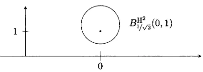
(3) 111. (see [5, Introductionl). Notice that the reght hand sides of these three equations have the following structure. some factor (. \displaystyle\frac{1}{2}|\vec{$\kap a$}|_{g}^{2}-$\lambda$+ sectional curvature),. since the sectional curvatures in \mathbb{H}^{2} , the Euclidean space and the sphere are respectively -1,. 0 and 1.. The article is structured as follows. In the next section we recall some basic facts on. the geometry of the hyperbolic plane. In Section 3 Proposition 1.1 is proven. In the last section we compare the elastic flow in \mathbb{H}^{2} for $\lambda$=0 and the Willmore flow of surfaces of revolution and show, by a direct computation, that they differ only by the factor 2 f_{2}^{4}.. 2. The geometry of the hyperbolic plane In this article we consider the Poincaré half‐plane model for the hyperbolic space, i.e.. the Riemannian manifold. (\mathbb{H}^{2}, g). with. \mathbb{H}^{2}=\{(y_{1}, y_{2})\in \mathbb{R}^{2} : y_{2}>0\}. and. g_{(y_{1},y_{2})=\displayst le\frac{1}y_{2}^{2}\left(\begin{ar y}{l 1&0\ 0&1 \end{ar y}\right). It is well known that (\mathbb{H}^{2}, g) has constant sectional curvature equal to symbols of (\mathbb{H}^{2}, g) are given by the following expressions. $\Gamma$_{11}^{1}=$\Gamma$_{22}^{1}=0,. $\Gam a$_{12}^{1}=$\Gam a$_{21}^{1}=-\displaystyle\frac{1}{y_{2} , $\Gam a$_{1 }^{2}=\displaystyle\frac{1}{y_{2}, $\Gam a$_{2 }^{2}=-\displaystyle\frac{1}{y_{2}. and. -1 .. .. The Christoffel. $\Gamma$_{12}^{2}=$\Gamma$_{21}^{2}=0.. Identifying \partial_{y_{1} with ( 1, 0)^{t} and \partial_{y_{2} with (0,1)^{t} one easily verifies the following formula for the covariant derivative in \mathbb{H}^{2}. \nabl _{\parti l_{x}fX=\left(\begin{ar y}{l \parti l_{x}X_{1}-\frac{1}f_{2}(X_{\mathrm{l}\parti l_{x}f_{2}+X_{2}\parti l_{x}f_{1})\ \parti l_{x}X_{2}+\frac{1}f_{2}(X_{1}\parti l_{x}f_{1}-X_{2}\parti l_{x}f_{2}) \end{ar y}\right). (2.1). for a vector field X along a curve f= (f_{1}, f_{2}):\mathrm{S}^{1} \rightar ow \mathbb{H}^{2} . Since we will consider geodesic circles in \mathbb{H}^{2} the following remark will be useful.. Remark 2.1 ([2, Proposition 2.6]). The geodesic distance between (x_{1}, y_{1}) , (x_{2}, y_{2})\in \mathbb{H}^{2} is given by dist \mathbb{H}^{2}. ( x_{1},y_{1}), (x_{2},y_{2}) =. In particular, if x_{1}. =x_{2}=x ,. arccosh. (1+\displaystyle \frac{(x_{2}-x_{1})^{2}+(y_{2}-y_{1})^{2} {2y_{2}y_{1} ). then \mathrm{d}\mathrm{i}\mathrm{s}\mathrm{t}_{\mathbb{H}^{2} ( x, y_{1}), (x, y_{2}) =. .. |\displaystyle \log_{y}^{y}\frac{2}{1}|.. By this formula it is easy to see that a ball in \mathbb{H}^{2} coincides with an Euclidean ball and vice versa, as shown in the following lemma. In Figure 1 (an isometry of) the circular limit curve from Proposition 1.1 is sketched.. Lemma 2.1. Let r, y_{1} >0 and x_{1} \in \mathbb{R} . Let B_{r}^{\mathbb{H}^{2} (x_{1}, y_{1}) be a ball in the hyperbolic plane defined by B_{r}^{\mathbb{H}^{2}}(x_{1}, y_{1})=\{(x, y)\in \mathbb{H}^{2} : dist\mathbb{H}^{2}((x,y), (x_{1}, y_{1}))<r\} . Then. B_{r}^{\mathbb{H}^{2} (x_{1}, y_{1})=B_{\sinh(r)y_{1} ^{\mathbb{R}^{2} (x_{1}, y_{1}\cosh(r). ,.

(4) 112. 0. Figure 1: The ball of radius 1/\sqrt{2} and midpoint (0,1) in the hyperbolic plane. where B_{ $\rho$}^{\mathb {R}^{2} (a) denotes the ball of radius Conversely for y_{1} >r>0 we find. $\rho$. and center. a. in the Euclidean plane \mathb {R}^{2} \supset \mathbb{H}^{2}.. B_{r}^{\mathbb{R}^{2} (x_{1}, y_{1})=B_{\tanh^{-1}(r/y_{1})}^{\mathbb{H}^{2} (x_{1}, \sqrt{y_{1}^{2}-r^{2} ). .. Proof. Let (x, y) \in \mathbb{H}^{2} . Then, by Remark 2.1 above and the monotonicity of \cosh one sees that \backslash \prime(x, y)\in B_{r}^{\mathbb{H}^{2} (x_{1}, y_{1}) if and only if. \displaystyle \cosh(r)>1+\frac{(x-x_{1})^{2}+(y-y_{1})^{2} {2yy_{1} . By rearrenging the terms we see that this is equivalent to. 2yy_{1}\cosh(r)>(x-x_{1})^{2}+y^{2}+y_{1}^{2} (cosh2 (r)-\sinh^{2}(r) ), and hence to. sinh2(r) y_{1}^{2}>(x-x_{1})^{2}+(y-\cosh(r)y_{1})^{2}, that gives (x, y). \in. B_{\sinh(r)y_{1} ^{\mathbb{R}^{2} (x_{1}, y_{1}\cosh(r) .. the first part together with the fact that if and $\eta$\cosh(R)=y_{1} , whence. \tanh(R)=. \displayt e\frac{}y_1}. \in. (0,1). The second part of the lemma follows using. B_{r}^{\mathbb{R}^{2} (x_{1}, y_{1}). and hence. =. B_{R}^{\mathbb{H}^{2} (x_{1}, $\eta$) ,. then r=\sinh(R) $\eta$. R=\tanh^{-1}(r/y_{1}). Similarly we find. $\eta$= \displaystyle \frac{y_{1} {\cosh(R)}=y_{1}\sqrt{1-(r/y_{1})^{2} = \sqrt{y_{1}^{2}-r^{2} . \square. 3. The elastic flow of circles in the hyperbolic plane. In this section, we study the evolution of circles under the elastic flow in the hyperbolic plane. Since we will consider a family of parametrised curves f f(x, t) whose time‐ derivative \partial_{t}f is not necessarily normal to \partial_{x}f we will work with the following flow instead =. of (1.3). We consider. \left\{ begin{ar y}{l (\partial_{t}f)^{\perp}=-\nabl _{L^2}\mathcal{E}_{$\lambda$}(f),&\mathrm{i}\mathrm{n}\mathrm{S}^{1}\times(0,T),\ f(x,0)=f_{0}(x),&\mathrm{f}\mathrm{o}\mathrm{r}x\in\mathrm{S}^{1}, \end{ar y}\right.. (3.1).

(5) 113. where. \perp. denotes the normal component Note that one can always transform a solution \mathb {R}/\mathb {Z} , ie via a. to (31) to a solution of (13) using the flow of vector fields on \mathrm{S}^{1} reparametrisation (see eg [6 \mathrm{p} 12] ). =. The following proposition gives a necessary and suffient condition under which a family. of circles is a solution to the elastic flow (31) Here and in the following we will always assume that f_{0} parametrises a geodesic circle in \mathbb{H}^{2} $\iota$\mathrm{e} by Lemma 21 we may assume that. \left(bgin{ar y}{l 0\ a_{0} \end{ar y}\ight) +r_{0}\left(\begin{ar y}{l \mathrm{c}\mathrm{o}\mathrm{s}(x)\ mathrm{S}1\mathrm{n}(x) \end{ar y}\right). f_{0}(x)= Proposition 3.1. for some. a_{0}. (32). >r_{0}>0. Let $\lambda$\in \mathbb{R} and 0<T\leq\infty. a_{0} 1 Let a(t) [0, T ) \rightarrow \mathbb{R}, r(t) [0, T ) \rightarrow \mathbb{R} be smooth functions satesfying a(0) r(0) =r_{0} and a(t) > r(t) > 0 for all 0 \leq t < T If the following family of curves =. f \mathrm{S}^{1} \times[0, T)\rightarrow \mathbb{H}^{2}. f(x, t)=. is a solution to (31) (0, \infty). w $\iota$ th. \left(\begin{ar y}{l 0\ a(t) \end{ar y}\right) +r(t)\left(\begin{ar y}{l \mathrm{c}\mathrm{o}\mathrm{s}x\ mathrm{S}\mathrm{l}\mathrm{n}x \end{ar y}\right). (33). initial value f_{0} as an (32) then $\rho$(t). is a solution to the ODE. =. \displaystle\frac{(t)}{r(t)} [0, T ). \left{\begin{ar y}{l \frac{\mathrm{d}\mathrm{d}t$\rho$(t)=H_{$\lambda$}( \rho$)\ $\rho$(0)=$\rho$_{0} \end{ar y}\right. where. H_{ $\lambda$}( $\rho$). =-\displaystyle \frac{1}{2} $\rho$($\rho$^{2}-1)($\rho$^{2}-2( $\lambda$+1)). and $\rho$_{0}. \rightarrow. (34). =\displaystyle \frac{a_{0} {r_{0} >1. 2 Moreover $\iota$ fp [0, T ) \rightarrow(0, \infty) $\iota$ s a smooth solute on to (34) with $\rho$_{0}>1 , then wreting $\rho$_{0}=a_{0}/r_{0} with a_{0}>r_{0}>0 there exist uneque smooth functions a, r [0, T ) \rightarrow(0, \infty) satesfying a(0) =a_{0} r(0) =r_{0} and a(t) > r(t) > 0 for all 0 \leq t < T , such that f (gvven by (33)) $\iota$ s a solution to (31) with initeal value f_{0} from (32) 3 For all $\lambda$\in \mathbb{R} and to (34) 4 If. $\rho$_{0} > 1. there exists a unaque smooth soluteon. -\displaystyle\frac{1}{2} then the smooth solution =\sqrt{2( $\lambda$+1)}. $\lambda$>. $\mu$_{ $\lambda$}. $\rho$. [0, \infty ). \rightarrow. $\rho$. [0, \infty ). \rightarrow. (1, \infty). (1, \infty) converges monotonecally to. The last part of the statement yields the existence of circular self similar solutions to the elastic flow, and these circles converge monotonically to the circle with constant. curvature. $\mu$_{ $\lambda$}. (see below). Corollary 3.1 For any $\lambda$\in \mathbb{R} and any emtial value f_{0} as an (32) there exists a famaly (33) of circles that satisfies the elastzc flow (31) Moreover for $\lambda$ > -\displaystyle \frac{1}{2} this famaly converges to the circle whech is given by. \displaystyle \frac{a}{r}=$\mu$_{ $\lambda$}=\sqrt{2( $\lambda$+1)} If $\lambda$\displaystyle \leq-\frac{1}{2} then the cercular self‐svmilar solutzon still exest but the czrcles expand to infinity as. t\rightarrow\infty. Note that this corollary and Lemma 21 immediately imply Proposition 11.

(6) 114. Proof. The first part of this corollary follows from the third and second claim of Proposition 3.1. The statement for $\lambda$>-\displaystyle \frac{1}{2} is also given in Proposition 3.1 whereas for $\lambda$\displaystyle \leq-\frac{1}{2} Lemma. A. 1 gives a solution. of (3.4) that converges asymptotically from above to. $\rho$. $\rho$= 1 .. For the. associated circular solution f this means that the quotient a/r converges to 1 and hence the circular solutions converge to a circle touching tangentially the line \{(x, 0) : x \in \mathbb{R}\} \square (see Lemma 2.1), i.e. expanding to infinity. The proof of Proposition 3.1 is given after the next lemmata. Note that the condition f is a well defined circle in \mathbb{H}^{2}.. a>r>0 ensures that. Lemma 3.1. For the circular curve f from (3.3) wzth. |\tilde{ $\kappa$}(x)|_{g}= \underline{a}. a>r>0. it holds (3.5). ’. r. -\displaystyle\nabla_{L^{2}\mathcal{E}_{$\lambda$}(f)=-($\lambda$+1-\frac{1}{2}\frac{a^{2}{r^{2})(a+r\sinx)\frac{a}{r \left(\begin{ar ay}{l \mathrm{c}\mathrm{o}\mathrm{s}x\ \mathrm{s}\mathrm{i}\mathrm{n}x \end{ar ay}\right) . In particular, f is an elastic curve if and only if Proof. We have. \partil_{x}f=r\left(\begin{ar y}{l -\mathrm{s}\mathrm{i}\mathrm{n}x\ \mathrm{c}\mathrm{o}\mathrm{s}x \end{ar y}\right). $\lambda$>-\displaystyle \frac{1}{2}. and. (3.6). \displaystyle \frac{a}{r}=\sqrt{2( $\lambda$+1)}.. , whence. |\displaystyle \partial_{x}f|_{g}=\frac{1}{f_{2} |\partial_{x}f|_{euc}=\frac{r}{a+r\sin x} (that is well defined since. a>r>0 ). and thus for the arc length derivative \partial_{s}=. we find. The tangential vector is. and from (2.1) we find. \nabla_{\partial_{\mathrm{s}}f}X=\partial_{s}X+ for vector fields. X. =. \displaystyle\frac{1}{|\partial_{x}f|_{q} \partial_{x}. \displaystyle \partial_{s}=\frac{1}{r}(a+r\sin x)\partial_{x}=\frac{f_{2} {r}\partial_{x}.. \partial_{\mathrm{s}f=(a+r\sinx)\left(\begin{ar y}{l -\mathrm{s}\mathrm{i}\mathrm{n}x\ \mathrm{c}\mathrm{o}\mathrm{s}x \end{ar y}\right). \left(begin{ar y}{l -X_{1}\mathrm{c}\mathrm{o}\mathrm{s}x+X_{2}\mathrm{s}\mathrm{i}\ athrm{n}x\ -X_{\mathrm{l}\mathrm{s}\mathrm{i}\ athrm{n}x-X_{2}\mathrm{c}\mathrm{o}\mathrm{s}x \end{ar y}\right). =\partial_{s}X-. \left(begin{ar y}{l X_{1}\mathrm{c}\mathrm{o}\mathrm{s}x-X_{2}\mathrm{s}\mathrm{i}\ athrm{n}x\ X_{1}\mathrm{s}\mathrm{i}\ athrm{n}x+X_{2}\mathrm{c}\mathrm{o}\mathrm{s}x \end{ar y}\right). (3.7). (X_{1}, X_{2}) along f . Using this formula we compute the curvature. vector field. \vec{ $\kappa$}(x)=\nabla_{\partial_{ $\varepsilon$}f}\partial_{\mathrm{s} f. =\displayst le\frac{ +\mathrm{r}\sinx}{\mathrm{r}\parti l_{x}[(a+r\sinx)\left(\begin{ar y}{l -\mathrm{s}\mathrm{i}\mathrm{n}x\ \mathrm{c}\mathrm{o}\mathrm{s}x \end{ar y}\right)]+(a r\sinx)\left(\begin{ar y}{l \mathrm{s}\mathrm{i}\mathrm{n}x\mathrm{c}\mathrm{o}\mathrm{s}x+\mathrm{c}\mathrm{o}\mathrm{s}x\mathrm{s}\mathrm{i}\mathrm{n}x\ \mathrm{s}\mathrm{i}\mathrm{n}^{2}x-\mathrm{c}\mathrm{o}\mathrm{s}^{2}x \end{ar y}\right) rrsin x)^{2}\left(begin{ar y}{l -\mathrm{c}\mathrm{o}\mathrm{s}x\ -\mathrm{s}\mathrm{i}\ athrm{n}x \end{ar y}\right) =(a+r\sinx)\cosx\left(\begin{ar ay}{l -\mathrm{s}\mathrm{i}\mathrm{n}x\ \mathrm{c}\mathrm{o}\mathrm{s}x \end{ar ay}\right) +\underline{(a+} +(a r\sinx)\left(\begin{ar y}{l 2\mathrm{s}\mathrm{i}\mathrm{n}x\mathrm{c}\mathrm{o}\mathrm{s}x\ \mathrm{s}\mathrm{i}\mathrm{n}^{2}x-\mathrm{c}\mathrm{o}\mathrm{s}^2}x \end{ar y}\right) x)^{2} rrsin \left(bgin{ary}l \mathr{c}\mathr{o}\mathr{s}x\ mathr{s}\mathr{i}\mathr{n}x \ed{ary}\ight) =(a+r\sinx)\left(\begin{ar y}{l \mathrm{s}\mathrm{i}\mathrm{n}x\mathrm{c}\mathrm{o}\mathrm{s}x\ \mathrm{s}\mathrm{i}\mathrm{n}^{2}x \end{ar y}\right) -\underline{(a+} =-(a+r\displayst le\sinx)\frac{ }r \left(\begin{ar y}{l \mathrm{c}\mathrm{o}\mathrm{s}x\ \mathrm{s}\mathrm{i}\mathrm{n}x \end{ar y}\right)..

(7) 115. Thus,. |\displaystyle \vec{ $\kappa$}|_{g}=\frac{1}{a+r\sin x}\cdot\frac{a}{r}\cdot(a+r\sin x)=\frac{a}{r},. that is (3.5). Using (3.7) again we find for \vec{ $\kappa$}=(\vec{ $\kappa$}_{1},\vec{ $\kappa$}_{2}) that. \left(bgin{ary}l \vec{$kap $}_{1\mathr{c}\mathr{o}\mathr{s}x-\vec{$kap $}_{2\mathr{s}\mathr{i}\mathr{n}x\ vec{$\kap $}_{1\mathr{s}\mathr{i}\mathr{n}x+\vec{$kap $}_{2\mathr{c}\mathr{o}\mathr{s}x \end{ary}\ight) =-\displayst le\frac{1}r(a+r\sinx)\partial_{x}[(a+r\sinx)\frac{a}r \left(\begin{ar y}{l \mathrm{c}\mathrm{o}\mathrm{s}x\ \mathrm{s}\mathrm{i}\mathrm{n}x \end{ar y}\right)]+(a+r\sinx)\frac{a}r\left(\begin{ar y}{l \mathrm{c}\mathrm{o}\mathrm{s}^{2}x-\mathrm{s}\mathrm{i}\mathrm{n}^{2}&x\ 2\mathrm{c}\mathrm{o}\mathrm{s}x\mathrm{s}\mathrm{i}\mathrm{n}x& \end{ar y}\right) =-\displaystyle \frac{1}{r}(a+r\sin x) [acosx \left(bgin{ary}l \mathr{c}\mathr{o}\mathr{s}x\ mathr{s}\mathr{i}\mathr{n}x \ed{ary}\ight) +(a r\displayst le\sinx)\frac{ }r\left(\begin{ar y}{l -\mathrm{s}\mathrm{i}\mathrm{n}x\ \mathrm{c}\mathrm{o}\mathrm{s}x \end{ar y}\right) ] +(a r\displaystle\sinx)\frac{}r\left(\begin{ar y}{l \mathrm{c}\mathrm{o}\mathrm{s}^2x-\mathrm{s}\mathrm{i}\mathrm{n}^2x\ 2\mathrm{c}\mathrm{o}\mathrm{s}x\mathrm{s}\mathrm{i}\mathrm{n}x \end{ar y}\right) =-(a+r\displaystyle \sin x)\frac{a}{r}(_{\cos x\sin x+(\frac{a}{r}\cos x+\sin x\cos x)-2\sin x\cos x}\cos^{2}x-(\frac{a}{ $\Gamma$}\sin x+\sin^{2}x)-(\cos^{2}x-\sin^{2}x) =-(a+r\displaystyle\sinx)\frac{a}{r}(_{\frac{a}{r}\cosx}^{-\frac{a}{r}\sinx})=(a+r\sinx)\frac{a^{2} {r^{2} \left(\begin{ar ay}{l \mathrm{s}\mathrm{i}\mathrm{n}x\ -\mathrm{c}\mathrm{o}\mathrm{s}x \end{ar ay}\right) \partil_{x}f=r\left(\begin{ar y}{l -\mathrm{s}\mathrm{i}\mathrm{n}x\ \mathrm{c}\mathrm{o}\mathrm{s}x \end{ar y}\right). \nabla_{\partial_{s}f}\vec{ $\kappa$}=\partial_{s}\vec{ $\kappa$}-. is tangential to f , i.e. a multiple of. . Thus. (\nabla_{\partial_{\mathrm{s} f})^{\perp}\vec{ $\kappa$}=0 and hence. ( \nabla_{\partial_{s}f})^{\perp})^{2}\vec{ $\kappa$}=0. Summarising, we find. -\displaystyle\nabla_{L^{2} \mathcal{E}_{$\lambda$}(f)=-(\nabla_{\partial_{s}f ^{\perp})^{2}\vec{$\kap a$}-\frac{1}{2}|\vec{$\kap a$}|_{g}^{2}\vec{$\kap a$}+\vec{$\kap a$}+$\lambda$\vec{$\kap a$}. =(-\displaystyle\frac{1}{2}|\vec{$\kap a$}|_{g}^{2}+$\lambda$+1)\vec{$\kap a$} =-($\lambda$+1-\displaystyle\frac{1}{2}\frac{a^{2}{r^{2})(a+r\sinx)\frac{a}{r\left(\begin{ar ay}{l \mathrm{c}\mathrm{o}\mathrm{s}x\ \mathrm{s}\mathrm{i}\mathrm{n}x \end{ar ay}\right),. that is (3.6). Since a>r>0 then \nabla_{L^{2} \mathcal{E}_{ $\lambda$}(f)=0 only when the quotient a/r is constant and equal to \sqrt{2( $\lambda$+1)} . Since the quotient has to be bigger than one, this can only be the case. when. $\lambda$. is strictly bigger than − \displayt e\frac{1}2 . This yields the claim.. \square. Lemma 3.2. Let $\lambda$\in \mathbb{R}, f_{0} given by (3.2) and f be as m(3.3) . Then f:\mathrm{S}^{1}\times[0, T ) \rightar ow \mathbb{H}^{2} is a solution to the elastic flow (3.1) if and only if the functions a, r : [0, T ) \rightar ow \mathbb{R} satisfy. \left\{ begin{ar y}{l \frac{\dot{a} r\sinx+\frac{\dot{r} =\frac{ }r(\frac{ }r+\sinx)(\frac{1}2(\frac{ }r)^{2}-($\lambda$+1) ,t>0,x\in\mathb {R},\ \frac{ (0)}{r(0)}=\frac{ _0}{r_0}, \end{ar y}\right.. where the dot represents the time derivative of a and. r.. (3.8).

(8) 116. Proof. For (\partial_{t}f)^{\perp} we calculate. and thus, since. N. :=. \partil_{t}f=\left(\begin{ar y}{l \dot{r}&\mathrm{c}\mathrm{o}\mathrm{s}x\ \dot{a}+\dot{r}&\mathrm{s}\mathrm{i}\mathrm{n}x \end{ar y}\right) \left(begin{ar y}{l \mathrm{c}\mathrm{o}\mathrm{s}x\ mathrm{s}\mathrm{i}\ athrm{n}x \end{ar y}\right)\per\partil_{x}f \left(bgin{ary}l 0\ dot{a} \end{ary}\ight) we find \partial_{t}f=. +rN and hence, using. \displaystyle\left(\begin{ar ay}{l 0\ \mathrm{l} \end{ar ay}\right)=\{ left(\begin{ar ay}{l 0\ \mathrm{l} \end{ar ay}\right),N\rangle_{f(x)}\cdot\frac{N}{|N_{f(x)}^{2} =\frac{(a+r\sinx)^{2} {(a+r\sinx)^{2} (\sinx)N=(\sinx)N we find. (\partial_{t}f)^{\perp}=(\dot{a} \sin x+r)N. Thus, together with (3.6) this shows that f from (3.3) is a solution to (3.1) if and only if. (\displaystyle \dot{a} \sin x+r)N=-( $\lambda$+1-\frac{1}{2}\frac{a^{2} {r^{2} ) (a+r\sin x)\frac{a}{r}N, i.e.. \displaystyle \frac{\dot{a} {r}\sin x+\frac{\dot{r} {r}=-\frac{a}{r}(\frac{a}{r}+\sin x) ( $\lambda$+1-\frac{1}{2}\frac{a^{2} {r^{2} ). .. Taking the initial values into account this yields the system (3.8).. \square. Proof of Proposition 3.1. We use here several times Lemma 3.2.. 1. Let f from (3.3) be a solution to the elastic flow with initial value f_{0} as in (3.2). Then, by the pr&evious lemma, the functions 0<r<a are solutions to (3.8). Differentiating (3.8) with respect to x yields. \displaystyle \frac{\dot{a} {r}\cos x=\frac{a}{r} (\frac{1}{2}(\frac{a}{r})^{2}-( $\lambda$+1) \cos x for all. x. , in particular for. x=0. we find. \displaystyle \dot{a}=a(\frac{1}{2}(\frac{a}{r})^{2}-( $\lambda$+1) .. (3.9). Plugging this equation into (3.8) yields. \displaystyle \dot{r}=a(\frac{a}{r}+\sin x)(\frac{1}{2}(\frac{a}{r})^{2}-( $\lambda$+1)) -a(\frac{1}{2}(\frac{a}{r})^{2}-( $\lambda$+1))\sin x =\displaystyle \frac{a^{2} {r}(\frac{1}{2}(\frac{a}{r})^{2}-( $\lambda$+1) .. Thus the function $\rho$. :=. \displayte\frac{} satisfies $\rho$(0)= \displayte\frac{}\mathr{g}\mathr{o} and. \displaystyle\dot{$\rho$}=\frac{\dot{a}{r}-\frac{a\dot{r}{r^2}. = \displaystyle \frac{a}{r} (\frac{1}{2} (\frac{a}{r})^{2}-( $\lambda$+1) -\frac{a^{3} {r^{3} (\frac{1}{2}(\frac{a}{r})^{2}-( $\lambda$+1). =-\displaystyle \frac{1}{2} $\rho$($\rho$^{2}-2( $\lambda$+1))($\rho$^{2}-1)=H_{ $\lambda$}( $\rho$). ..

(9) 117. 2. Conversely, let a_{0}. >. r_{0}. >. 0.. $\rho$. be the solution to \dot{$\rho$}. Then. $\rho$ >. 1. =. H_{ $\lambda$}( $\rho$) and $\rho$(0). =. by Lemma A.l. Moreover, let. for some \ d i s p l a y t e \ f r a c { _ 0 } { r } be the solution to. $\rho$_{0}. a. =. the linear ODE. \left\{ begin{ar ay}{l \dot{a}=a\cdot\frac{1}{2}($\rho$^{2}-2($\lambda$+1) ,t>0\ a(0)=a_{0} \end{ar ay}\right. and define. r. by r(t). $\rho$(t)=\displaystyle \frac{a(t)}{r(t)} for all. t\in. \displayst le\frac{ (t)}{$\rho$(t)} . Then [0, T ). Moreover, :=. a a. >. 0. since. a_{0}. >. 0,. (3.10) thus. r. >. 0. and hence. satisfies (3.10), whence. \displaystyle\frac{\dot{r}{r}=\frac{\mathrm{d}{\mathrm{d}t\logr =\displaystyle\frac{\mathrm{d} {\mathrm{d}t \loga-\frac{\mathrm{d} {\mathrm{d}t \log$\rho$. =\displaystle\frac{\dot{a} -\frac{\dot{$\rho$}{$\rho$}. =\displaystyle \frac{1}{2} ( \frac{a}{r})^{2}-2( $\lambda$+1) -\frac{r}{a}H_{ $\lambda$}(\frac{a}{r}) =\displaystyle \frac{1}{2} ( \frac{a}{r})^{2}-2( $\lambda$+1)) +\frac{1}{2}( \frac{a}{r})^{2}-2( $\lambda$+1)) ( \frac{a}{r})^{2}-1) =\displaystyle \frac{1}{2} ( \frac{a}{r})^{2}-2( $\lambda$+1) (\frac{a}{r})^{2} which shows that. \displaystyle \frac{\dot{a} {r}\sin x+\frac{\dot{r} {r}=\frac{a}{r}(\frac{1}{2}(\frac{a}{r})^{2}-( $\lambda$+1) \sin x+\frac{1}{2}( \frac{a}{r})^{2}-2( $\lambda$+1) (\frac{a}{r})^{2} =\displaystyle \frac{a}{r}(\frac{a}{r}+\sin x) (\frac{1}{2}(\frac{a}{r})^{2}-( $\lambda$+1) ,. i.e. (3.8) holds. Lemma 3.2 implies the rest of the claim. 3. The last two assertions follow from Lemma A.l.. 4. \square. Relationship to the Willmore flow of surfaces of rev‐. olution It is well known (see e.g. [10, 11]) that there is a very interesting relation between the. 0 ) of curves in the hyperbolic half plane and the elastic energy \mathcal{E} (that is \mathcal{E}_{$\lambda$} with $\lambda$ Willmore energy of surfaces of revolution. As a consequence the two gradient flows are =. also closely related as observed in [6]. Here, we give the detailed computations to see that the two differ only by a factor when we take into account that the Willmore flow keeps the rotationally symmetry. We shortly fix some notation to state the result. Let f : \mathrm{S}^{1} \rightarrow \mathb {R}_{+}^{2} := \{(x, z)^{t} : z > 0\} be a closed curve parametrised by Euclidean arc‐length, i.e. (f_{1}')^{2}+(f_{2}')^{2} \equiv 1 . By rotating the curve around the x‐axis we obtain a surface of revolution in \mathbb{R}^{3}. h_{f} : \mathrm{S}^{1}\times [0, 2 $\pi$]\ni(x, $\varphi$)\mapsto(f_{1}(x), f_{2}(x)\cos( $\varphi$), f_{2}(x)\sin( $\varphi$))^{t}\in \mathbb{R}^{3}.

(10) 118. Its Willmore energy is given by. W(h_{f})=\displaystyle \int H^{2}\mathrm{d}S, f can be considered as a curve in \mathbb{H}^{2} . In order to stress this fact we denote it as f_{\mathb {H}^{2} . Similarly, when needed, we write f_{\mathb {R}^{2} to indicate that f is now considered as a curve in \mathbb{R}^{2}. with H the mean curvature. The same curve. Theorem 4.1. One has. 1. \mathcal{E}(f_{\mathbb{R}^{2} )= \displaystyle \frac{2}{ $\pi$}W (hf); 2. the L^{2} ‐gradient of \mathcal{E} satisfy. \nabla_{L^{2}}\mathcal{E}(f_{\mathbb{H}^{2}})=-2f_{2}^{4}(\triangle H+2H(H^{2}-K))\vec{n}_{\mathbb{R}^{2}} where we recall that.. \nabla_{L^{2}}W(h_{f})=( $\Delta$ H+2H(H^{2}-K))\vec{N} with \vec{n}_{\mathbb{R}^{2} = ( f_{2}' , ‐fí) and \vec{N}=(f_{2}' , ‐fí \cos( $\varphi$) , ‐fí \sin( $\varphi$)) ; 3. the elastic flow can be written as. (\partial_{t}f_{\mathbb{H}^{2} )^{\perp}=-\nabla_{L^{2} \mathcal{E}(f_{\mathbb{H}^{2} )=2f_{2}^{3}( $\Delta$ H+2H(H^{2}-K))\vec{n}_{\mathbb{H}^{2} =-2f_{2}^{4}( $\Delta$ H+2H(H^{2}-K))\vec{n}_{\mathbb{R}^{2}}. The last part of the statement gives the relation between the elastic flow and the Willmore flow of surfaces of revolution. Of course we cannot compare directly these two flows since one lives in \mathbb{H}^{2} while the other takes place in \mathbb{R}^{3} . On the other hand, as we will explain below, when we start from a surface of revolution this symmetry is preserved by the Willmore flow and hence we can describe the Willmore flow simply considering the evolution of the generating curve in \mathbb{R}^{2} . This is the flow that differ by a factor 2 f_{2}^{4} from the elastic flow in \mathbb{H}^{2}.. Proof. Relation between the energies This is well known and can be found for instance. in [10, 11, 4, 3]. We repeat the arguments. The first fundamental form of the surface of revolution h_{f} is given by. I=\left(\begin{ar y}{l 1&0\ 0&f_{2}^{2} \end{ar y}\right). ,. the induced area element is f_{2}\mathrm{d}x\mathrm{d} $\varphi$ , the normal vector is. \vec{N}= (f_{2}' , ‐fí \cos( $\varphi$), -f_{1}'\sin( $\varphi$))^{t},. the principal curvatures are curvatures are respectively. $\lambda$_{1} =f\'{i}' f_{2}'-f_{2}'' fí. H=\displaystyle \frac{1}{2} (f_{1}'f_{2}' - f2\displaystyle \prime\prime f_{1}'+\frac{f_{1}' {f_{2} ). and. and. $\lambda$_{2}. K=. =. ( fí’. \displayte\frac{}f’\mathr{L}2 and the mean and Gauss. f_{2}'-f_{2}'f_{1}')\displaystyle \frac{f_{1}' {f_{2} .. (see [7, page 161]) and the Willmore energy of this surface of revolution is given by. W(h_{f})=\displaystyle \int H^{2}\mathrm{d}S=\frac{ $\pi$}{2}\int_{\mathrm{S}^{1} (f_{1}' f_{2}'-f_{2}' fí \displayst le\frac{f_1}'{f_2})^{2}f_{2} d +. x. ..

(11) 119. Now we consider the same curve as a curve. f : \mathrm{S}^{1} \rightar ow \mathbb{H}^{2}, f=f_{\mathbb{H}^{2}} . Since this curve is. parametrised by Euclidean arc‐length we find. \displaystyle \partial_{s}f=\frac{1}{|\partial_{x}f|_{g} \partial_{x}f=f_{2}\partial_{x}f. and. \partial_{s}=f_{2}\partial_{x}.. For the ‘hyperbolic’ curvature from (2.1) we find \vec{ $\kappa$}=\nabla_{s}\partial_{s}f= and. \left(\begin{ar y}{l \partil_{s}^2f_{1}-&\frac{2}f_{2}\partil_{s}f 1}\partil_{s}f 2}\ \frac{1}f_{2}\partil_{s}^2f_{2}+(\partil_{s}f 1})^{2}&-(\partil_{s}f 2})^{2}) \end{ar y}\right) \left(\begin{ar y}{l f_{2}^ \partil_{x}^2f_{1}-f_{2}\partil_{x}f 1\partil_{x}f 2\ f_{2}^ \partil_{x}^2f_{}+f_{2}(\partil_{x}f 1)^{2} \end{ar y}\right) =. (4.1). |\displaystyle \vec{ $\kap a$}|_{g}^{2}=\frac{1}{f_{2}^{2} [ (f_{2}^{2}f_{1}' -f_{2}f\'{i} f_{2}')^{2}+(f_{2}^{2}f_{2}' +f_{2}(f_{1}')^{2})^{2}]. =f_{2}^{2}[(f_{1}'-\displaystyle \frac{f_{1}' {f_{2} f_{2}')^{2}+(f_{2}' +\frac{(f_{1}')^{2} {f_{2} )^{2}] =f_{2}^{2}[(f_{1}')^{2}+\displaystyle \frac{(f_{1}')^{2}(f_{2}')^{2} {f_{2}^{2} -2 í’ \displaystyle \frac{f_{1}' {f_{2} f_{2}'+(f_{2}')^{2}+\frac{(f_{1}')^{4} {(f_{2})^{2} +2f_{2}'\frac{(f_{1}')^{2} {f_{2} ] f. which, using that f satisfies (f_{1}')^{2}+(f_{2}')^{2}\equiv 1 and hence fí( x ) f_{1}''(x)+f_{2}'(x)f_{2}''(x)=0 ,. (4.2). can be rewritten as. |\displaystyle \vec{ $\kap a$}|_{g}^{2}=f_{2}^{2}[(f_{1}'f_{2}'-f_{2}'f_{1}')^{2}+\frac{(f_{1}')^{2} {f_{2}^{2} -2f_{1}'\frac{f_{1}' {f_{2} f_{2}'+2f_{2}'\frac{(f_{1}')^{2} {f_{2} ] =f_{2}^{2} [ ( í’ f_{2}'-f_{2}' f_{1}'+\displaystyle \frac{f_{1}' {f_{2} )^{2}-4 í’ \displaystyle\frac{f_{1}' {f_{2} f_{2}'+4f_{2}'\frac{(f_{1}')^{2} {f_{2} ] =f_{2}^{2}[ (f_{1}' f_{2}'-f_{2}' f\displaystyle \'{i}+ \frac{f_{1}' {f_{2} )^{2}+\frac{4f_{2}' }{f_{2} ]. f. f. This formula gives directly the relation between the elastic energy in the hyperbolic plane and the Willmore energy of surfaces of revolution, indeed since the curve is closed. \displaystyle \mathcal{E}(f_{\mathb {H}^{2} )=\int_{\mathrm{S}^{1} |\vec{ $\kap a$}|_{9}^{2}\frac{1}{f_{2} \mathrm{d}x=\int_{\mathrm{S}^{1} [(f_{1}'f_{2}'-f_{2}'f\'{i}+ \frac{f_{1}' {f_{2} )^{2}+\frac{4f_{2}' {f_{2} ]f_{2}\mathrm{d}x =\displaystyle \frac{2}{ $\pi$}W(h_{f})+4\int_{\mathrm{S}^{1} f_{2}'(x)\mathrm{d}x=\frac{2}{ $\pi$}W ( hf ). Notice that here. \mathcal{E}(f). denotes. \mathcal{E}_{ $\lambda$}(f) with $\lambda$=0. The Willmore flow starting from a surface of revolution The Willmore flow of. h_{f} is given by. (\partial_{t}h_{f})^{\perp}=-\nabla_{L^{2}}W(h_{f})=-(\triangle H+2H(H^{2}-K))\vec{N} ,. (4.3). with \vec{N} the normal to the surface as fixed before and \triangle the Laplace‐Beltrami operator.. Blatt in [1] proved that the Willmore flow, as long as it exists, keeps its rotational sym‐ metry. Hence we can restrict the flow directly on the \{(x, z):z>0\} plane (or take $\varphi$=0 in the rotation) and obtain that the right hand side of (4.3) so restricted is given by. -( $\Delta$ H+2H(H^{2}-K))(f_{2}', -f_{1}')^{t}.

(12) 120. Hence, by taking into account this rotational invariance, the Willmore flow corresponds to the following flow equation for the evolving curve in \mathbb{R}^{2}. (\partial_{t}f_{\mathbb{R}^{2}})^{\perp}=-( $\Delta$ H+2H(H^{2}-K))\vec{n}_{\mathbb{R}^{2}}, with. \vec{n}_{\mathbb{R}^{2}}=(f_{2}', -f_{1}')^{t}.. We compute now $\Delta$ H+2H(H^{2}-K) . We do the computations locally where f_{2}'\neq 0,. so that using again (4.2) in the form of. f_{2}' =-\displaystyle \frac{f_{1}'f_{1}' }{f_{2} we have. H=\displaystyle \frac{1}{2} (\displaystyle\frac{f_ 1}' {f_ 2} +\frac{f_ 1}' {f_ 2} ). and. K=\displaystyle\frac{f_{1}'f_{1}' {f_{2}f_{2} .. Note that a similar formula holds where f\'{i}\neq 0 , see [4]. By a direct computation (using (4.2) several times). 2 $\Delta$ H=2\displaystyle \frac{1}{f_{2} \partial_{x}(f2\partial_{x}H). =\displaystyle\partial_{x}(\frac{f_{1}^{(3)}{f_{2}-\frac{f_{1}'f_{2}' {(f_{2}')^{2}+\frac{f_{1}' {f_{2}-\frac{f_{1}'f_{2}'{f_{2}^{2})+\frac{f_{2}'{f_{2}(\frac{f_{1}^{(3)}{f_{2}-\frac{f_{1}'f_{2}' {(f_{2}')^{2}+\frac{f_{1}' {f_{2}-\frac{f_{1}'f_{2}'{f_{2}^{2}) =\displaystyle\partial_{x}(\frac{f_{1}^{(3)} {f_{2} +\frac{(f_{1}')^{2}f_{1}' {(f_{2})^{3} +\frac{f_{1}' {f_{2} -\frac{f_{1}'f_{2}' {f_{2}^{2} )+\frac{f_{2}' {f_{2} (\frac{f_{1}^{(3)} {f_{2} +\frac{(f_{1}')^{2}f_{1}' {(f_{2})^{3} +\frac{f_{1}' {f_{2} -\frac{f_{1}'f_{2}' {f_{2}^{2} ). =\displaystyle\frac{f_{1}^{(4)} {f_{2} -\frac{f_{1}^{(3)} {(f_{2}')^{2} f_{2}'+2\frac{f_{1}^{(3)}f_{1}'f_{1}' {(f_{2})^{3} +\frac{(f_{1}')^{3} {(f_{2}')^{3} -3\frac{(f_{1}')^{2}f_{1}'f_{2}' {(f_{2}')^{4} +\displaystyle\frac{f_{1}^{(3)} {f_{2} -\frac{f_{1}'f_{2}' {f_{2}^{2} -\frac{f_{1}'f_{2}' {f_{2}^{2} -\frac{f_{1}'f_{2}' {f_{2}^{2} +2\frac{f_{1}'(f_{2}')^{2} {f_{2}^{3} +\frac{f_{1}^{(3)} {f2}+\frac{(f_{1}')^{2}f_{1}' {f_{2}(f_{2}')^{2} +\frac{f_{1}'f_{2}' {f_{2}^{2} -\frac{f_{1}'(f_{2}')^{2} {f_{2}^{3} =\displaystyle\frac{f_{1}^{(4)} {f_{2} +3\frac{f_{1}^{(3)}f_{1}'f_{1}' {(f_{2})^{3} +2\frac{f_{1}^{(3)} {f_{2} +\displaystyle \frac{(f_{1}')^{3} {(f_{2}')^{3} +3\frac{(f_{1}')^{3}(f_{1}')^{2} {(f_{2}')^{5} -\frac{f_{1}'f_{2}' {f_{2}^{2} +\frac{(f_{1}')^{2}f_{1}' {f_{2}'f_{2}^{2} +\frac{f_{1}'(f_{2}')^{2} {f_{2}^{3} +\frac{(f_{1}')^{2}f_{1}' {f_{2}(f_{2}')^{2}. whereas. 2H(H^{2}-K)= (\displaystyle \frac{f_{1}'}{f_{2}' +\frac{f_{1}' {f_{2} )(\frac{1}{4}(\frac{f_{1}'}{f_{2}' +\frac{f_{1}' {f_{2} )^{2}-\frac{f_{1}'f_{1}' {f_{2}f_{2}' ) =\displaystyle\frac{1}{4}(\frac{f_{1}' {f_{2}' +\frac{f_{1}' {f_{2} )(\frac{f_{1}' {f_{2}' -\frac{f_{1}' {f_{2} )^{2}. (4.4). The elastic flow We consider now the gradient flow for the elastic energy in the hyperbolic half‐plane. (\displaystyle\partial_{t}f_{\mathb {H}^{2} )^{\perp}=-(\nabla_{s}^{\perp})^{2}\vec{$\kap a$}-\frac{1}{2}|\vec{$\kap a$}|_{g}^{2}\tilde{$\kap a$}+\vec{$\kap a$}.. Working again locally where f_{2}'\neq 0 using (4.2) we can rewrite the curvature (see (4.1)) as \vec{ $\kappa$}=. ( -\displayst le\frac{f_ 2}f_{1}' {f_ 2}' fí) \vec{n}_{\mathbb{R}^{2}, +. with \vec{n}_{1\mathrm{H}^{2} the normal vector in the hyperbolic half plane given by. \vec{n}_{\mathbb{H}^{2}}=f_{2}(-\partial_{x}f_{2}, \partial_{x}f_{1})=-f_{2}\vec{n}_{\mathbb{R}^{2}}..

(13) 121. Hence it has the same direction as the normal vector to the curve. f_{\mathb {R}^{2} in the Euclidean. plane but it differs by a factor of -f_{2}. Since \nabla_{s}\vec{n}_{\mathbb{H}^{2} is tangential, we directly obtain that. \nabla_{s}^{\perp}\vec{ $\kappa$}=f_{2}\partial_{x} ( =f_{2}. -\displayst le\frac{f_2}f_{1}' {f_2}'. í) \vec{n}_{\mathb {H}^{2}. +f. (— fí’ -\displaystyle \frac{f_ 2}f_{1}^{(3)} {f_ 2}' +\frac{f_ 2}f_{1}' {(f_{2}')^{2} f_{2}' +fí’) \vec{n}_{\mathb {H}^{2}. =(-\displaystyle\frac{f_{2}^{2}f_{1}^{(3)} {f_{2}' -\frac{f_{2}^{2}f_{1}'(f_{1}')^{2} {(f_{2}')^{3} )\vec{n}_{\mathb {H}^{2} and similarly. (\displaystyle\nabla_{s}^{\perp})^{2}\vec{$\kap a$}=f_{2}\partial_{x}(-\frac{f_2}^{2}f_{1}^{(3)}\prime}{f_2}'-\frac{f_2}^{2}f_{1}'(f_{1}')^{2}{(f_{2})^{3})\vec{n}_{\mathb {H}^{2} =f_{2}(-\displaystyle \frac{f_{2}^{2}f_{1}^{(4)} {f_{2}' -2f_{2}f_{1}^{(3)}+\frac{f_{2}^{2}f_{1}^{(3)} {(f_{2}')^{2} f_{2}'-2\frac{f_{2}f_{1}'(f_{1}')^{2} {(f_{2})^{2} -\frac{f_{2}^{2}(f_{1}')^{3} {(f_{2}')^{3} -2\displaystyle\frac{f_{2}^{2}f_{1}'f_{1}'f_{1}^{(3)} {(f_{2}')^{3} +3\frac{f_{2}^{2}f_{1}'(f_{1}')^{2} {(f_{2}')^{4} f_{2}')\vec{n}_{\mathb {H}^{2} =f_{2}(-\displaystyle \frac{f_{2}^{2}f_{1}^{(4)} {f_{2}' -2f_{2}f_{1}^{(3)}-3\frac{f_{2}^{2}f_{1}^{(3)} {(f_{2}')^{3} f_{1}' \displaystyle\frac{f_2}f_{1}'(f_{1}')^{2}{(f_{2})^{2}-\frac{f_2}^{2}(f_{1}')^{3}{(f_{2}')^{3} fí—2. -3\displaystyle\frac{f_{2}^{2}(f_{1}')^{2}(f_{1}')^{3}{(f_{2}')^{5})\vec{n}_{\mathb {H}^{2}. using (4.4), whereas. \displaystyle\frac{1}{2}|\vec{$\kap a$}|_{9}^{2}\vec{$\kap a$}-\vec{$\kap a$}=\frac{1}{2}(-\frac{f_{2}f_{1}' {f_{2}' +f_{1}')^{3}\vec{n}_{\mathb {H}^{2-} (-\frac{f_{2}f_{1}' {f_{2}' +f_{1}')\tilde{n}_{\mathb {H}^{2} =-\displaystyle\frac{1}{2}f_{2}^{3}(\frac{f_{1}' {f_{2}' -\frac{f_{1}' {f_{2} )^{3}\vec{n}_{\mathb {H}^{2-} ( -\displayst le\frac{f_2}f_{1}' {f_2}' í) =-4f_{2}^{3}H(H^{2}-K)+f_{2}^{3}(\displaystyle \frac{f_{1}'}{f_{2}' -\frac{f_{1}' {f_{2} )^{2}\frac{f_{1}' {f_{2} \vec{n}_{\mathb {H}^{2} + ( \displaystle\frac{f_2}f_{1}'{f_2}' — +f. One sees that the first three terms in terms in 2\triangle H.. \vec{n}_{\mathb {H}^{2}. í) \vec{n}_{\mathbb{H}^{2}.. f. (\nabla_{s}^{\perp})^{2}\vec{ $\kap a$} differ only by a factor from the first three. Relation between the L^{2} ‐gradients and the gradient flows Comparing the ex‐ pression we see that. -(\displaystyle\partial_{t}f_{\mathb {H}^{2} )^{\perp}=\nabla_{L^{2} \mathcal{E}(f_{\mathb {H}^{2} )=(\nabla_{s}^{\perp})^{2}\vec{$\kap a$}+\frac{1}{2}|\tilde{$\kap a$}|_{g}^{2}\vec{$\kap a$}-\vec{$\kap a$}. =-f_{2}^{3}(\displaystyle \frac{f_{1}^{(4)} {f_{2} +2\frac{f_{1}^{(3)} {f_{2} +3\frac{f_{1}^{(3)} {(f_{2}')^{3} f_{1}'f_{1}'+2\frac{f_{1}'(f_{1}')^{2} {f_{2}(f_{2}')^{2} +\frac{(f_{1}')^{3} {(f_{2})^{3} +3\frac{(f_{1}')^{2}(f_{1}')^{3} {(f_{2}')^{5}. +4H(H^{2}-K)- (\displaystyle \frac{f_{1}' {f_{2}' -\frac{f_{1}' {f_{2} )^{2}\frac{f_{1}' {f_{2} -\frac{f_{1}' {f_{2}'f_{2}^{2} +\frac{f_{1}' {f_{2}^{3} )\vec{n}_{\mathb {H}^{2} =-f_{2}^{3}(2 $\Delta$ H-\displaystyle \frac{(f_{1}')^{3} {(f_{2})^{3} -3\frac{(f_{1}')^{3}(f_{1}')^{2} {(f_{2}')^{5} +\frac{f_{1}'f_{2}' {f_{2}^{2} -\frac{(f_{1}')^{2}f_{1}' {f_{2}'f_{2}^{2} -\frac{f_{1}'(f_{2}')^{2} {f_{2}^{3} -\frac{(f_{1}')^{2}f_{1}' {f_{2}(f_{2})^{2}.

(14) 122. +2\displaystyle\frac{f_{1}'(f_{1}')^{2} {f_{2}(f_{2}')^{2} +\frac{(f_{1}')^{3} {(f_{2}')^{3} +3\frac{(f_{1}')^{2}(f_{1}')^{3} {(f_{2}')^{5} +4H(H^{2}-K)- (\displaystyle \frac{f_{1}' {f_{2} -\frac{f_{1}' {f_{2} )^{2}\frac{f_{1}' {f_{2} -\frac{f_{1}' {f_{2}'(f_{2})^{2} +\frac{f_{1}' {f_{2}^{3} )\vec{n}_{\mathb {H}^{2} =-f_{2}^{3}(2\displaystyle \triangle H+\frac{f_{1}'f_{2}' {f_{2}^{2} -\frac{(f_{1}')^{2}f_{1}' {f_{2}'f_{2}^{2} -\frac{f_{1}'(f_{2}')^{2} {f_{2}^{3} +\frac{(f_{1}')^{2}f_{1}' {f_{2}(f_{2}')^{2} +4H(H^{2}-K)-(\displaystyle \frac{f_{1}' {f_{2} -\frac{f_{1}' {f_{2} )^{2}\frac{f_{1}' {f_{2} -\frac{f_{1}' {f_{2}'(f_{2})^{2} +\frac{f_{1}' {f_{2}^{3} )\vec{n}_{\mathb {H}^{2} =-f_{2}^{3}(2 $\Delta$ H-2\displaystyle \frac{(f_{1}')^{2}f_{1}' {f_{2}'f_{2}^{2} +\frac{(f_{1}')^{3} {f_{2}^{3} +\frac{(f_{1}')^{2}f_{1}' {f_{2}(f_{2}')^{2} +4H(H^{2}-K)- (\displaystyle \frac{f_{1}' {f_{2}' -\frac{f_{1}' {f_{2} )^{2}\frac{f_{1}' {f_{2} )\vec{n}_{\mathb {H}^{2}. =-2f_{2}^{3}(\triangle H+2H(H^{2}-K) \vec{n}_{\mathbb{H}^{2} =2f_{2}^{4}(\triangle H+2H(H^{2}-K) \vec{n}_{\mathbb{R}^{2} =-2f_{2}^{4}(\partial_{t}f_{\mathrm{R}^{2} )^{\perp} Hence the two flows differ by the factor 2 f_{2}^{4}.. \square. Acknowledgement Anna Dall’Acqua would like to thank Shinya Okabe for the invitation to Sendai and. Kyoto and the nice discussions. Adrian Spener is supported by the DFG (project number 355354916).. A. Analysis of the ordinary differential equation. Here, we shortly study the ODE for the curvature $\rho$= \displaytle\frac{}r . We remind the reader that we define $\mu$_{ $\lambda$} := \sqrt{2( $\lambda$+1)} for $\lambda$>-\displaystyle \frac{1}{2} , see Proposition 3.1. Lemma A.l. Let $\rho$. $\lambda$ \in \mathbb{R}. : [0, \infty)\rightarrow(1, \infty) to (3.4),. and. $\rho$ 0. i.e .. to. >. 1.. There exists a unique global smooth solution. \left\{ begin{ar y}{l \frac{\mathrm{d}{\mathrm{d}t $\rho$(t)=H_{$\lambda$}($\rho$)=-\frac{1}2 $\rho$(p^{2}-1)($\rho$^{2}- ($\lambda$+1)\ $\rho$(0)=$\rho$_{0}. \end{ar y}\right. Depending on $\lambda$ , we have the following asymptotic behaviour of $\rho$ : 1. If. $\lambda$>-\displaystyle \frac{1}{2} ,. then the solution. $\rho$. satisfies. (i) if $\rho$(0)>$\mu$_{ $\lambda$} , then p(t)\searrow$\mu$_{ $\lambda$} as t\rightarrow\infty, (ii) if $\rho$(0)<$\mu$_{ $\lambda$} , then p(t)\nearrow$\mu$_{ $\lambda$} as t\rightarrow\infty. 2. If. $\lambda$\displaystyle \leq-\frac{1}{2} ,. then $\rho$(t)\searrow 1 as. t\rightarrow\infty.. Proof. Existence and uniqueness of a global solution follow from smooothness of the right. hand side and the existence and uniqueness theory of autonomous ODEs (see e.g. [15]). Concerning the asymptotic behavior, for $\lambda$>-\displaystyle \frac{1}{2} we have $\mu$_{ $\lambda$}>1 , and hence H_{ $\lambda$}( $\rho$) >0 for 1< $\rho$<$\mu$_{ $\lambda$} as well as H_{ $\lambda$}(p)<0 for $\rho$>$\mu$_{ $\lambda$} (see Figure 2). In the case of $\lambda$\displaystyle \leq-\frac{1}{2} we have H_{ $\lambda$}( $\rho$)<0 for any $\rho$> 1 , and since H_{ $\lambda$}(1)=0 we find $\rho$>1 for all times 0\leq t<\infty. \square.

(15) 123. Figure 2: The graph of H_{ $\lambda$} for. $\lambda$>-\displaystyle \frac{1}{2}.. References [1] BLATT, S. A singular example for the Willmore flow. Analyses (Munich) 29, 4 (2009), 407‐430.. [2] BRIDSON, M. R., AND HAEFLIGER, A. Metrt,c spaces of non‐positive curvature, vol. 319 of Grundlehren der Mathematischen Wissenschaften [Fundamental Principles of Mathematical Sciencesl. Springer‐Verlag, Berlin, 1999.. [3] BRYANT, R., AND GRIFFITHS, P. Reduction for constrained variational problems and \displaystyle \int\frac{1}{2}k^{2}ds . Amer. J. Math. 108, 3 (1986), 525‐570. [4] DALL’ACQUA, A., DECKELNICK, K., AND GRUNAU, H.‐C. Classical solutions to the Dirichlet problem for Willmore surfaces of revolution. Adv. Calc. Var. 1, 4 (2008), 379‐397.. [5] DALL’ACQUA, A., LAUX, T., LiN, C.‐C., Pozzi, P., AND SPENER, A. The elastic flow of curves in the sphere. J. Diff. Flow (to appear) (2017). [6] DALL’ACQUA, A., AND SPENER, A. The elastic flow of curves in the hyperbolic plane. Preprent (https://arxiv.org/abs/1710.09600) (2017).. [7] DO CARMO, M. P. Differential geometry of curves and surfaces. Prentice‐Hall, Inc., Englewood Cliffs, N.J., 1976. Translated from the Portuguese.. [8] DZIUK, G., KUWERT, E., AND SCHÄTZLE, R. Evolution of elastic curves in existence and computation. SIAM J. Math. Anal. 33, 5 (2002), 1228‐1245.. \mathbb{R}^{n} :. [9] Koiso, N. On the motion of a curve towards elastica. In Actes de la Table Ronde de Géométrie Différentielle (Luminy, lg92), vol. 1 of Sémin. Congr. Soc. Math. France, Paris, 1996, pp. 403‐436.. [10] LANGER, J., AND SINGER, D. Curves in the hyperbolic plane and mean curvature of tori in 3‐space. Bull. London Math. Soc. 16, 5 (1984), 531‐534.. [11] LANGER, J., AND SINGER, D. A. The total squared curvature of closed curves. J. Differential Geom. 20, 1 (1984), 1‐22. [12] MARQUES, $\Gamma$ . C., AND NEVES, A. Min‐max theory and the Willmore conjecture. Ann. of Math. (2) 179, 2 (2014), 683‐782. [13] NOVAGA, M., AND OKABE, S. Curve shortening‐straightening flow for non‐closed planar curves with infinite length. J. Differential Equations 256, 3 (2014), 1093‐1132. [14] SZENTHE, J. On the total curvature of closed curves in Riemannian manifolds. Publ. Math. Debrecen 15 (1968), 99‐105..

(16) 124. [15] TESCHL, G. Ordinary differential equations and dynamical systems, vol. 140 of Grad‐ uate Studaes in Mathematics. American Mathematical Society, Providence, RI, 2012.. [16] TSUKAMOTO, Y. On the total absolute curvature of closed curves in manifolds of negative curvature. Math. Ann. 210 (1974), 313‐319. [17] WEN, Y. L^{2} flow of curve straightening in the plane. Duke Math. J. 70, 3 (1993), 683‐698.. Anna Dall’Acqua, Adrian Spener, Universität Ulm, HelmholtzstraBe 18, 89081 Ulm, Germany, anna.dallacqua@uni‐ulm.de, adrian. spener@uni‐ulm.de,.

(17)