Strichartz estimates for wave equations in the homogeneous Besov space (Harmonic Analysis and Nonlinear Partial Differential Equations)

Strichartz estimates for wave equations

in the homogeneous Besov space

M.Nakamura (中村誠)

Department ofMathematics, _HokkaidoUniversity

1

Introduction

In this note the author describes his recent work on the linear

esti-mates for wave equations inthe homogeneous Besov space. We consider the inhomogeneous

wave

equations

$\partial_{t}^{2}u(t, x)-\triangle u(\mathrm{t}, X)=f(t, x)$, $t\in \mathrm{R},$ $x\in \mathrm{R}^{n},$ $n\geq 2$,

(1.1)

$u(\mathrm{O}, x)=\partial_{t}u(0, x)=0$,

where $n$ denotes the space dimension, $f$ is a complex valued function on

$\mathrm{R}\cross \mathrm{R}^{n}$, and $\triangle$ denotes the Laplacian inspace variables. We shall prove

Strichartz estimates of the following type

$||u;L^{q}(I,\dot{B}_{r}^{\rho},)2||\leq C||f;L^{\tilde{q}}(I,\dot{B}_{\tilde{r},2}\tilde{\rho})||$, (1..2)

where $I$ denotes an interval in $\mathrm{R},\dot{B}_{r,2}^{\rho}$ denotes the homogeneous Besov space defined later and the constant $C$ is independent of $f$ and $I$

.

For

any $1\leq q\leq\infty$ and a Banach space $X$, we write the mixed norm of a

function $g:Iarrow X$ by

$||g;L^{q}(I, x)||= \{\int_{t\in I}||g(t);X||^{q}dt\}^{1/}q$ for $1\leq q<\infty$,

(1.3)

$||g;L \infty(I, X)||=\sup_{t\in I}||g(\mathrm{t});^{x}||$.

On the estimate (1.2), Ginibre and Velo in [3] have shown

some

generalization of almost all Strichartz-type estimates obtained uptothat point, in which one of conditions necessary for (1.2) is given by

$\rho+\delta(r)-1/q=2+\tilde{\rho}+\delta(\tilde{r})-1/\tilde{q}$, $\rho,\tilde{\rho}\in \mathrm{R}$, (1.4)

where $\delta(r)=n(1/2-1/r)$ (see [3, Proposition 3.1]). On the other

hand, Harmse in [5], Oberlin in [10], Bak, $\mathrm{M}\mathrm{c}\mathrm{M}\mathrm{i}\mathrm{C}\mathrm{h}\mathrm{a}\mathrm{e}\mathrm{l}$ and Oberlin in

[1] have already shown the ”off duality” estimates, namely (1.2) for $(n+1)/2n-2/(r\iota+1)<1/r<(n-1)/2n$ with $q=r,\tilde{q}=\tilde{r}$ and $\rho=\tilde{\rho}=0$ in (1.4). The above two results meet only on the original

The author introduce Strichartz estimates which involve the above results and have new ones. Although the proofs

are

omitted, they

are

obtained by the abstract setting such as the unitarity of the operator

$\exp(it\sqrt{-\triangle})(i=\sqrt{-1})$ , the duality argument, the

Hardy-Littlewood-Sobolev inequality and the complex interpolation method. The key method is complex $\mathrm{i}\mathrm{n}\mathrm{t}\mathrm{e}\mathrm{r}\mathrm{p}_{0}1\mathrm{a}\mathrm{t}\mathrm{i}\mathrm{o}\mathrm{n}(\mathrm{s}\mathrm{e}\mathrm{e}$ [$2$, Chapter 4] or Proposition 2.

1 below), by which we could loosen the conditions restricted by the

$\mathrm{H}\mathrm{a}\mathrm{r}\mathrm{d}\mathrm{y}- \mathrm{L}\mathrm{i}\mathrm{t}\mathrm{t}\mathrm{l}\mathrm{e}\mathrm{w}\mathrm{o}\mathrm{o}\mathrm{d}-\mathrm{s}_{0}\mathrm{b}\mathrm{o}\mathrm{l}\mathrm{e}\mathrm{v}$inequality, therefore

our

results could involve

[1, Theorem 6’], [5, Theorem 2.3] and [10, Theorem 3].

Our main result is Proposition 2. 2. Recently Keel and Tao [7]

have obtained the estimate at the ”endpoint” by the real interpolation

method. We used their methods to supplement our methods in the

crit-ical cases.

2

Notation

and

propositions

As usually done, we will rewrite (1.1) to the $\mathrm{i}\mathrm{n}\mathrm{t}\mathrm{e}_{\circ}\sigma\Gamma \mathrm{a}1$ equation. For that purpose, we introduce some operators defined on the tempered

dis-tributions $S’(\mathrm{R}n)$ or$S’(\mathrm{R}\cross \mathrm{R}n)$

.

Wedenote by$\omega^{\lambda},$ $U(t)$ theoperators on

$S’(\mathrm{R}^{n})$ defined by $\omega^{\lambda}=(-\triangle)^{\lambda/2},$ _{$U(t)=\exp(i,t\sqrt{-\Delta})$}, and by _{$c_{0},$}$c_{\pm}$

the integral operators $\mathrm{d}\mathrm{e}\mathrm{f}\mathrm{i}_{\mathrm{I}1}\mathrm{e}\mathrm{d}$by

$G_{0}f(t)= \int_{0}^{t}U(t-s)f(s)dS$, $G_{\pm}f(t)= \int_{\pm\infty}^{t}U(t-s)f(s)dS$, (2.5)

for any function $f$ in$S’(\mathrm{R}^{n+1})$

.

We denote by $G$ any of $G_{0},$ $G_{\pm}$, and by

$H$ the operator $\omega^{-1}G$. To show the required inequality (1.2), it suffices

to show the boundedness of the operator $H$ from $L^{\tilde{q}}(\mathrm{R},\dot{B}^{\tilde{\rho}}(\tilde{r},2\mathrm{R}n))$ to

$L^{q}(\mathrm{R},\dot{B}^{\rho}(r,2\mathrm{R}n))$.

Here we shall introduce the homogeneous Besov space $\dot{B}_{r,s}^{\rho}(\mathrm{R}^{n})$ for

any $\rho\in \mathrm{R}$ and $1\leq r,$$s\leq\infty$ (see also [2], [3] and [12]). For $1\leq q\leq\infty$

andanormedspace$X$, we denoteby$\ell_{j}^{q}(X)$ the space of$\{a_{j}\}_{j\mathrm{z}}\in’ a_{j}\in X$,

with the

norm

given by

$||a_{j};ljq(X)||$ $=$ $\{\sum_{j\in \mathrm{Z}}||a_{j};X||q\}1/q$ for $1\leq q<\infty$,

(2.6)

$||a_{j};\ell_{j}\infty(X)||$ $=$ $\sup_{j\in \mathrm{Z}}||a_{j};X||$.

in space. Let $\{\varphi_{j}\}_{j\in}\mathrm{z}\subset C^{\infty}(\mathrm{R}^{n})$ such that

$\mathrm{s}\mathrm{u}\mathrm{p}\mathrm{p}F\varphi_{j}\subset\{x|2^{j-1}<|x|<2^{j+1}\}$,

$\sum_{j\in \mathrm{Z}}F\varphi j(x)=1$ for

$|x|\neq 0$

.

(2.7)

We denote by $\dot{B}_{r,s}^{\rho}(\mathrm{R}^{n})$ the space given by

$\{u\in S’(\mathrm{R}n)|||u;\dot{B}_{r,S}^{\rho}(\mathrm{R}^{n})||\equiv||2^{\rho j}\varphi j*u;\ell^{s}(jL^{r}(\mathrm{R}^{n}))||<\infty\}$

.

(2.8)

We make abbreviation such

as

$\dot{B}_{r}^{\rho}=\dot{B}_{r,2}^{\rho}(\mathrm{R}^{n})$ and $L^{q}\dot{B}_{r}^{\rho}=L^{q}(\mathrm{R},\dot{B}_{r}^{\rho})$

.

The main tools

are

embeddings($\mathrm{s}\mathrm{e}\mathrm{e}[2$, Theorem 6.5.1])

$\dot{B}_{r}^{0}arrow L^{r}$ for $2\leq r<\infty$, $L^{r_{\mathrm{L}}}arrow\dot{B}_{r}^{0}$ for $1<r\leq 2$, (2.9) $\dot{B}_{r}^{\rho}\llcorner_{arrow\dot{B}_{r_{1}}}\rho 1$ for $\rho\geq\rho_{1}$ with $\rho-n/r=\rho_{1}-n/r_{1}$, (2.10)

and the following complex interpolation method (see [2, Th 5.1.2, Th

6.4.5]). Let $\mu$ be

a

positive

measure

on

$\mathrm{R}$, and for any Banach space

$X$, let $L^{q}(\mathrm{R}, \mu;x)$ be the space ofa function $f$ : $\mathrm{R}arrow X$ with the norm $\{\int_{\mathrm{R}}||f;X||^{q}d\mu\}^{1}/q$ for _{$1\leq q<\infty$},

(2.11)

$\sup_{t\in \mathrm{R}}||f(t);x||$ for _$q=\infty$

.

Proposition 2. 1 Let $n\geq 1$

.

Let $1\leq s_{0},$$s_{1},$ $r_{0},$$r_{1}\leq\infty_{f}1\leq q_{0},$ $q_{1}<\infty$

and $\rho 0,$$\rho_{1}\in$ R. Let $K$ be an bounded operator

from

$L^{q_{0}}(\mathrm{R}, \mu;\dot{B}\rho 0)r_{0}$ to

$\dot{B}_{s_{0}}^{0}$, and

from

$L^{q_{1}}(\mathrm{R}, \mu;\dot{B}_{r_{1}}\rho_{1})$ to $\dot{B}_{s_{1}}^{0}$

.

Then $K$ is a bounded operator

from

$L^{q}(\mathrm{R}, \mu;\dot{B}_{r}\rho)$ to $\dot{B}_{s}^{0}$, where

$s,$ $r,$ $q,$$\rho$ are given by

$1/s=(1-\theta)/s_{0}+\theta/s_{1}$, $1/r=(1-\theta)/r_{0}+\theta/r_{1}$,

(2.12)

$1/q=(1-\theta)/q_{0}+\theta/q_{1}$, $\rho=(1-\theta)\rho 0+\theta\rho 1$,

for

any $0\leq\theta\leq 1$

.

In order to describe

our

statement in concise form, following Kato

[6], it is convenient to

use

the following geometric notation. We denote

by $\square$ the closed unit square in $\mathrm{R}^{2}$,

defined by $0\leq x,$ $y\leq 1$

.

In this

note we denote by $Q$ and $\tilde{Q}$ the points $(1/q, 1/r)$ and $(1/\tilde{q}, 1/\tilde{r})$ in $\square$

respectively, and we write $x(Q)=1/q,$ $y(Q)=1/r$. For $P,$ $Q\in\square$,

$[PQ]$ and $(PQ)$ represent the closed and open segment connecting $P$

and $Q$ respectively. And [$PQ)$ denotes $[PQ]\backslash \{Q\}$. We denote by $q’$ the

conjugate of $q$, namely $q’=q/(q-1)$ for $1<q\leq\infty$ and $q’=\infty$ for

points and sets in $\square$

,

by which it is convenient

to state

our

propositions

(see Figure 1,2,3).

$o=(\mathrm{o}, \mathrm{o})$, $A=(1,1)$, $B=(0,1/2)$, $C=(1/2, (n-3)/2(n-1))$,

$(C=(1/4,0)$ if$n=2$ ), $D=(1/2,0)$,

$E=(1, (n-3)/2(n-1))$, _{$F=(0, (n-3)/2(n-1))$},

( $E=D,$ $F_{--O}$ if _$n=2$ ),

$T_{0}=[OBCD]$ ($T_{0}=[OBC]$ if $n=2,$ $T_{0}=[OBC]\backslash \{C\}$ if$n=3$ ),

$T=\{B\}\cup(BEF)$,

(2.13)

where [OBCD] denotes the closure of the square defined by $\mathit{0},$ $B,$ $C_{\text{ノ}}$,

$D$, and _$(BEF)$ denotes the interior domain of the triangle defined

by $B$,

$E,$ $F$. For a set $S$ in $\square$, we denote by _$S’$

the set of the point $Q’$ with

$Q\in S$

.

Ifwe introduce the linear functionals

$\pi(Q)=1/r+2/(n-1)q$, $\pi_{1}(Q)=1/r+1/(n-1)q$_{, (2.14)}

for $Q$ in $\square$, then _$B$ and _$C$ are on

the line defined by $\pi(Q)=1/2,$ $B$ and $E$ are on _{$\pi_{1}(Q)=1/2,$ $B’$ and $C’$} are on _{$\pi(Q)=(n+3)/2(n-1),$}

$B’$ and $E’$ are on _{$\pi_{1}(Q)=(n+1)/2(n-1)$}

.

_{The pair $(Q,\tilde{Q})$ will}

be called a conjugate pair if $Q$ and $\tilde{Q}$ in $\square$ satisfy

$\pi(\tilde{Q})=\pi(Q)+2/(n-1)$

.

_(2.15)

In particular, for $Q\in[BC]$ and $\tilde{Q}\in[B’C’],$ $(Q,\tilde{Q})$ is

a

conjugate pair.

We

now

refer to the followingtwo properties. Let $(Q, Q’)$ be a conjugate

pair. If$x(Q)=0$ _and $x(\tilde{Q})=1$, then _{$y(Q)=y(\tilde{Q})$}

.

If_{$Q$ is} on _{[BE] and}

$x(\tilde{Q})=1$, then $y(Q’)=y(\tilde{Q})$

.

We callthepair $(Q,\tilde{Q})$ admissible if the linear operator_$H$is

bounded from $L^{\tilde{q}}\dot{B}_{\tilde{r}}^{\tilde{\rho}}$ to $L^{q}\dot{B}_{r}^{\rho}$ for any

$\rho$ and $\tilde{\rho}$ in $\mathrm{R}$such that

$\rho+\delta(r)-1/q=2+\tilde{\rho}+\delta(\tilde{r})-1/\tilde{q}$

.

(2.16)

Since $\omega^{\lambda}(\lambda\in \mathrm{R})$ is an isomorphism

from $\dot{B}_{r}^{\rho}$ to $\dot{B}_{r}^{\rho-\lambda}$, if the linear

operator $G$ is bounded from $L^{\tilde{q}}\dot{B}_{\tilde{r}}^{\tilde{\rho}}$ to $L^{q}\dot{B}_{r}^{\rho}$ for any

$\rho$ and $\tilde{\rho}$ in $\mathrm{R}$ such

that

$\rho+\delta(r)-1/q=1+\tilde{\rho}+\delta(\tilde{r})-1/\tilde{q}$, (2.17)

then $(Q,\tilde{Q})$ is admissible.

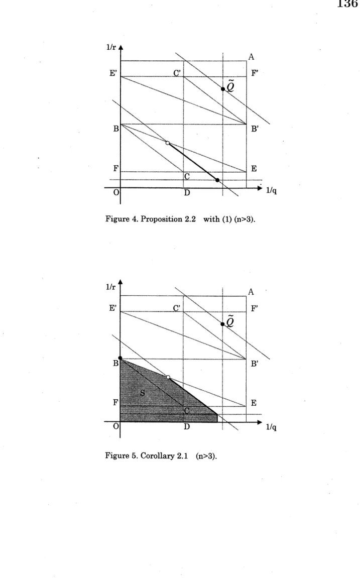
Proposition 2. 2 (see Figure 4) Let $n\geq 2$

.

Let $(Q,\tilde{Q})$ be a

conju-gatepairwith$x(Q)<x(\tilde{Q})$. And let$Q$ and$\tilde{Q}$ satisfy one

of

thefollowing

conditions.

(1) $\tilde{Q}\in T’,$ $(n-3)/(n-1)\tilde{r}’\leq 1/r$ ( $(n-3)/(n-1)\tilde{r}’<1/r$

for

$n=3$ ).

Moreover $\pi_{1}(Q)<1/2$ and $0<x(Q)$

if

$\tilde{Q}\not\in[B’C’)$

.

(2) $Q\in T_{f}1/\tilde{r}\leq 1-(\uparrow x-3)/(n-1)r(1/\tilde{r}<1-(n-3)/(n-.1)r$

for

$n=$

3).

Moreover $\pi_{1}(\tilde{Q})’\backslash >(n+1)/2(n-1)$ and $x(\tilde{Q})<1$

if

$Q\not\in[BC)$

.

Then the pair $(Q,\tilde{Q})$ is admissible.

Remark 1. Let $(Q,\tilde{Q})$ be an admissible pair with $\tilde{q}\neq\infty$ and $\tilde{r}\neq\infty$.

Then $(\tilde{Q}’, Q’)$ is also an admissible pair. Indeed, $H’$, the dual operator

of $H$, is a bounded operator from $L^{q’}\dot{B}_{r}^{-\rho}$, to $L^{\tilde{q}’}\dot{B}_{\tilde{r}}-,\tilde{\rho}$, and (2.16) could

be written as

$-\tilde{\rho}+\delta(\tilde{r}’)-1/\tilde{q}’=2-\rho+\delta(r’)-1/q’$

.

(2.18)

Since $H$ is written as a linear combination of $H_{0}’,$ $H_{\pm}’$, therefore $(\tilde{Q}’, Q’)$

is also

an

admissible pair. In this sense, the proof for the

case

(2) in

Proposition 2. 2 follows from that of (1) immediately.

Remark 2. In Proposition 2. 2, applying the Sobolev embedding the-orem,

we

could take $Q$ and $\tilde{Q}$ in $\square$

more

widely. For example, let

$(Q,\tilde{Q})$ be an admissible pair, then for any $r_{1},\tilde{r}_{1}$ with $0\leq 1/r_{1}\leq 1/r$

and $1/\tilde{r}\leq 1/\tilde{r}_{1}\leq 1,$ $((1/q, 1/r_{1}),$$(1/\tilde{q}, 1/\tilde{r}_{1}))$ is also an admissible

pair (note that the embeddings $\dot{B}_{r}^{\rho}\mathrm{L}arrow\dot{B}_{r_{1}}^{\rho_{1}}$ and $\dot{B}_{\tilde{r}_{1}}^{\tilde{\rho}_{1}}\mathrm{e}arrow\dot{B}_{\tilde{r}}^{\overline{\rho}}$ imply

$\rho+\delta(r)=\rho_{1}+\delta(r_{1})$ and $\tilde{\rho}+\delta(\tilde{r})=\tilde{\rho}_{1}+\delta(\tilde{r}_{1})$ in (2.16) respectively).

To show some typical examples the Sobolev embedding theorem

ap-plied to Proposition 2. 2, we introduce

a

set $S$ in $\square$

.

For $\tilde{Q}\in T’$, let $\nu$

be the supremum of $x(Q)$ with $(Q,\tilde{Q})$ in Proposition 2. 2 with (1). Let

now

$S$ be a set given by

$S\equiv$ $\{Q\in\square |\pi(\tilde{Q})\geq\pi(Q)+2/(n-1),$ $x(Q)<x(\tilde{Q})$,

$0<x(Q)\leq l^{\text{ノ}}$ ($0<x(Q)<\nu$ for $n=3$)$\}$ if $\tilde{Q}\in(B’C^{\prime_{E’}})$

,

$S\equiv$ _{$B\cup\{Q\in\square |\pi_{1}(Q)<1/2,$ $\pi(\tilde{Q})\geq\pi(Q)+2/(n-1)$},

$x(Q)\leq\nu$ ($x(Q)<\nu$ for $n=3$),$x(Q)<x(\tilde{Q})\}$ if $\tilde{Q}\in\tau’\backslash (B^{\prime_{C^{\prime_{E’}}}})$

.

For $Q\in T$, let $S$ be the set defined by $Q’$ as above, and let $S’$ be the set

of the point $Q_{1}’$ with $Q_{1}\in S$

.

Corollary 2. 1 (see Figure 5) Let $\tilde{Q}\in T’$ and _{$Q\in S$}

.

Or let _{$Q\in T$}

and $\tilde{Q}\in S’$

.

Then $(Q,\tilde{Q})i_{\mathit{8}}$ admissible.

Remark 3. The most familiar Strichartz-type estimates are the mixed

space-time estimates in the Lebesgue space. Ifthe conjugate pair $(Q,\tilde{Q})$

satisfies (2.16) with $\rho=\tilde{\rho}=0$, then it holds

$1/\tilde{r}-1/r=1/\tilde{q}-1/q=2/(n+1)$

.

_(2.20)

Therefore if $Q$ and $\tilde{Q}\mathrm{s}\mathrm{a}\mathrm{t}\mathrm{i}\mathrm{s}6^{r}(2.20)$ and (1) or (2) in Proposition 2. 2,

then we have

$||Hf;L^{q}L^{r}||\leq C||f,$ $L^{\tilde{q}}L\tilde{r}||$, (2.21) for any $f\in L^{\tilde{q}}L^{\tilde{r}}$, where we have used the embedding (2.9). Especially

for the diagonal case, namely $r=q$ and $\tilde{r}=\tilde{q}$,

we

obtain the estimate

given by [1, theorem 6’], [$\ulcorner)$, Theorem 2.3], [10,

Theorem 3]. Indeed for

$(n+1)/2n-2/(n+1)<1/r\leq(n-1)/2(n+1)$, the above $Q$ and$\tilde{Q}\mathrm{s}\mathrm{a}\mathrm{t}\mathrm{i}_{\mathrm{S}}6^{r}$

(1) in Proposition 2. 2, and for $(n-1)/2(n+1)<1/r<(n-1)/2n,$ $(2)$

in Proposition 2. 2. In the above argument, $Q$ is uniquely determined

by $\tilde{Q}$ as (2.20). But we $\mathrm{s}\mathrm{h}_{0}\mathrm{u}\mathrm{l}\mathrm{d}$ note that if _{$(Q,\tilde{Q})$}

in Corollary 2. 1 satisfies (2.16) with $\rho=\tilde{\rho}=0$, then (2.21) also holds.

In Proposition 2. 2, we must

assume

$x(Q)<x(\tilde{Q})$ and $x(Q)>0$,

or

$x(\tilde{Q})<1$

.

The following _{proposition could give}

some

_{supplements for}

the

cases

$x(Q)=x(\tilde{Q})=1/2,$ _{$x(Q)=0$ and} $x(\tilde{Q})=1$.

Proposition 2. 3 Let $2\leq r\leq\infty,$ $1\leq\tilde{q}\leq 2\leq q\leq\infty$

.

Let $\tilde{r}=r’$, and

let $\pi(\tilde{Q})>\pi(Q)+2/(n-1)$

.

_Then $(Q,\tilde{Q})$ is admissible.

The results in Proposition 2. 3 for the case $1<\tilde{q}<2<q<\infty$ are

also obtained by Corollary 2. 1 and Remark 2. Let now $\tilde{Q}$ be fixedwith $x(\tilde{Q})=1$, and let

$Q_{c}$ be the point such that

$\pi(\tilde{Q})=\pi(Qc)+2/(n-1)$ _{and $\pi_{1}(Q_{c})=1/2$}

.

_(2.22)

And let $T_{1},$ $S_{1}$ be the sets given by

$S_{1}\equiv T_{1}\cup\{Q\in\square |\pi_{1}(Q)<1/2, x(Q)<x(Q_{c}), x(Q)\leq 1/2\}$

.

(2.24)

For $Q$ with $x(Q)=0$, let $S_{1}$ be the set given by $Q’$

as

above, and let

S\’i

be the set of the point $Q_{1}’$ with $Q_{1}\in S_{1}$

.

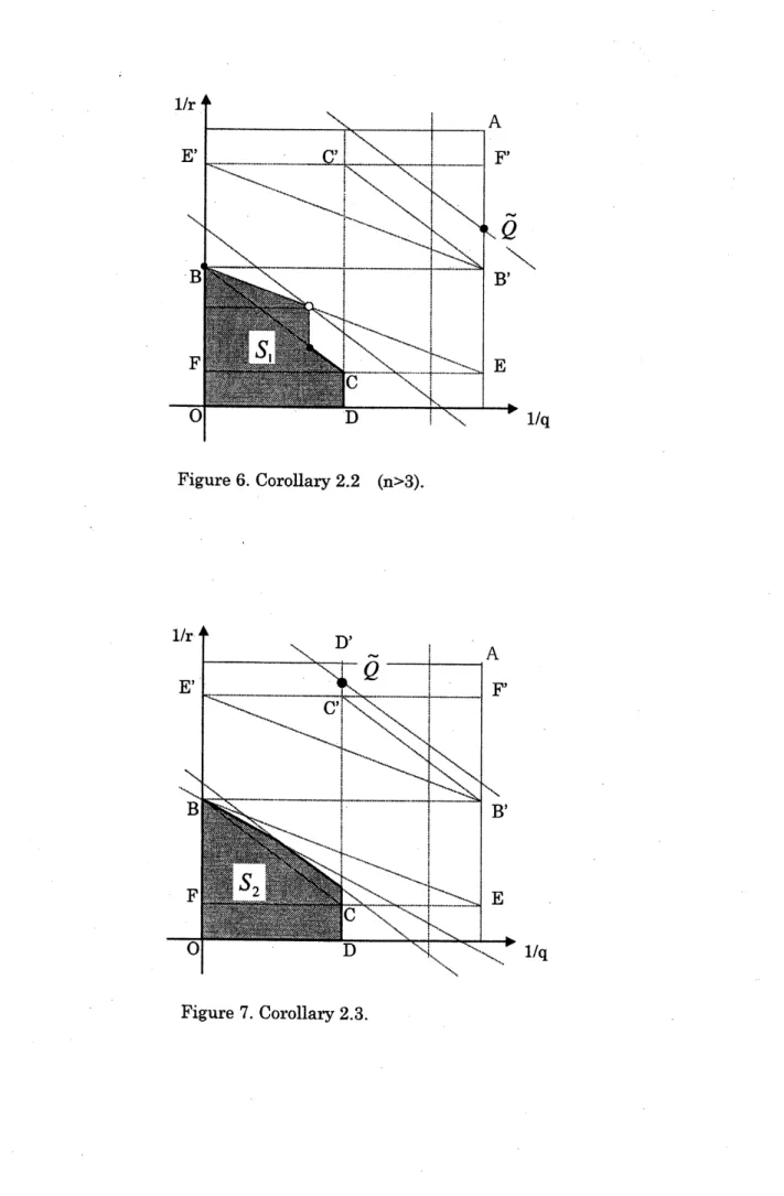
Corollary 2. 2 (see Figure 6) Let $1\leq\tilde{r}\leq 2,\tilde{Q}=(1,1/\tilde{r})$ and $Q\in S_{1}$. Or let $2\leq r\leq\infty,$ $Q=(0,1/r)$ and $\tilde{Q}\in S\text{\’{i}}.$ Then $(Q,\tilde{Q})$ is

$admis\mathit{8}ible$

.

Next

we

consider the case $q=\tilde{q}=2$ with $n\geq 4$

.

In this case,

applying Proposition 2. 3 and Remark 2,

we were

able to show the admissibility of $(Q,\tilde{Q})$ for any _$Q\in(CD$] and $\tilde{Q}\in(C’D’$]. However the

real interpolation method described in [7] could give

some

extension in

this

case.

Namely with the proof in [7, section 6] slightly modified,

we

obtain the following lemma.

Lemma 2. 1 Let $n\geq 4$

.

Let $(Q,\tilde{Q})$ be a conjugate pair.

If

$x(Q)=$

$x(\tilde{Q})=1/2$ and

$(n-1)/2(n-2)<y(\tilde{Q})<(n^{2}-_{\mathrm{t}}\ulcorner))/2(n-1)(n-2)$, _(2.25)

then $(Q,\tilde{Q})$ is admissible.

Since Lemma 2. 1 is obtained quite analogously to [7], we will use it

without proof. To proceed our argument, it is convenient to introduce

the linear functional

$\pi_{2}(Q)=1/r+1/(n-2)q$

.

_(2.26)

For $\tilde{Q}$ with $x(\tilde{Q})=1/2$, let

$T_{2},$ $S_{2}$ be sets given by

$T_{2}\equiv\{Q\in\square |\pi_{2}(Q)\leq 1/2, \pi(Q)\leq\pi(\tilde{Q})+2/(n-1), x(Q)\leq 1/2\}$,

(2.27)

$S_{2}\equiv T_{2}$ for $\tilde{Q}\in[C’D’]$, $S_{2}\equiv T_{2}\backslash [oB]$ for $\tilde{Q}\not\in[C’D’]$

.

(2.28)

For $Q$ with $x(Q)=1/2$, let $S_{2}$ be the set given by $Q’$ as above, and let

$S_{2}’$ be the set of the point $Q_{1}’$ with $Q_{1}\in S_{2}$.

Corollary 2. 3 (see Figure 7) Let $n\geq 4$. Let $\tilde{Q}\in\square$ satisfy $x(\tilde{Q})=$

$1/2$ and (2.25), and let $Q\in S_{2}$

.

Or let $Q\in\square$ satisfy $x(Q)=1/2$ and

$(n-3)^{2}/2(n-1)(n-2)<y(Q)<(n-3)/2(n-2)$, and let $\tilde{Q}\in S_{2}^{l}$

.

$1/\mathrm{q}$

Fifure 1. $\mathrm{n}>3$.

Fifure 2. $\mathrm{n}=3$.

Figure 4.Proposition 2.2 with (1)$(\mathrm{n}>3)$.

Figure6. Corollary 2.2 $(\mathrm{n}>3)$.

参考文献

[1] J.-G.Bak, D.McMichael, D.Oberlin, $L^{p_{-}}L^{q}$ estimates

off

the line

of

duality, J.Austral.Math.Soc. (Series A), 58(1995),

154-166.

[2] J.Bergh, J.L\"ofstr\"om, ”Interpolation Spaces,” Springer-Verlag, Berlin-Heidelberg-New York, 1976.

[3] J.Ginibre, G.Velo, Generalized Strichartz inequalities

_for

the wave

equation, J. Funct. Anal., 133(1995), 50-68.

[4] G.Hardy, $\mathrm{J}.\mathrm{E}$.Littlewood, G.P\’olya, ”Inequalities (Second

edi-tion),” Cambridge Mathematical Library,

1952.

[5] J.Harmse, On Lebesgue space estimates

_for

the wave equation,

In-diana Univ.Math.J., 39(1990), 229-248.

[6] T.Kato, An $L^{q,r}$-Theory

for

nonlinear $Sc\Gamma\ddot{O}dinger$ equations,

Ad-vanced Studies in Pure Math., 23(1994), 223-238.

[7] M.Keel, T.Tao, Endpoint $St7\dot{\mathrm{V}}ChartZ$ estimates, Amer.J.Math,

120(1998), 955-980.

[8] H.Lindblad, A sharp counterexample to the local existence

of

low-regularity solutions to nonlinear wave equations, Duke Math.J.,

72(1993), 503-539.

[9] M.Nakamura, T.Ozawa, The Cauchy problem

_for

nonlinear wave

equations in the homogeneous Sobolev space, Ann.Inst.Henri

Poincar\’e, Physique th\’eorique, (in press).

[10] D.Oberlin, Convolution estimates

_for

some distributions with

sin-gulanties on the light cone, Duke Math.J., 59(1989), 747-757.

[11] $\mathrm{R}.\mathrm{S}$.Strichartz, Restrictions

of

Fourier

_transforms

to quadratic

sur-$face\mathit{8}$ and decay

of

solutions

of

wave equations, Duke Math.J.,

44(1977), 705-714.

[12] H.hiebel, ”Interpolation Theory, Function Spaces, Differential