NOTE ON FLEX CURVES AND THEIR
APPLICATIONS
MUTSUO OKA
1.
INTRODUCTION
1.1. Let $f(x, y)\in \mathrm{C}[x, y]$ be a polynomial. We consider an affine curve $C^{a}(f):=\{(x, y)\in$ $\mathrm{C}^{2};f(x, y)=0\}$ and the projective curve $C(f)$ defined by the closure of
$C^{a}(f)$ in $\mathrm{P}^{2}$.
In this talk, we introduce the notion ofa flex curve of degree $\ell$, denoted by
$\mathcal{F}^{(l)}(f;P)$, at a
smooth point $P$ of a given curve $C^{a}(f)$.
As an application, we construct, in Section 5, another projective curve $C_{3}$ of degree 12 with
27 cusps for which $\pi_{1}(\mathrm{P}^{2}-C_{3})$ is abelian. The triple $\{C_{1}, C_{2}, c_{3}\}$ gives the first
example of
a triple of projective curves such that $\deg C_{i}=12,$ $i=1,2,3$ and they have 27 cusps but
their complements are topologically not homeomorphic. This implies that the moduli space of curvesof degree 12 with 27 cusps has at least 3 irreduciblecomponents. The pair $\{\mathit{0}_{1},\mathit{0}_{3}\}$ is of
particular interestto us as thecycliccovering argument (see for example [2]) cannot distinguish
$C_{1}$ and $C_{3}$ as their Alexander polynomials are trivial. 2. $\mathrm{c}_{\mathrm{Y}\mathrm{C}\mathrm{L}\mathrm{I}\mathrm{C}}\mathrm{c}\mathrm{o}\mathrm{v}\mathrm{E}\mathrm{R}\mathrm{I}\dot{\mathrm{N}}$
GS AND DISCRIMINANT POLYNOMIALS
We say that $f$ is a polynomial of type $(a, b;d)$ where $a,$$b$ are coprime positive integers if the
degree of$f(x, y)$ with weight$(X)=a$ and weight$(y)=b$is$d$
.
Wedenoteit by$\deg_{P}(f)=d$where$P:={}^{t}(a, b)$
.
We denote the set of such polynomials by $\mathcal{M}(a, b;d)$.
For a given $f\in \mathcal{M}(a, b;d)$,the$P$-principalpart at infinity of$f$ is defined by thesum of the monomials in
$f(x, y)$ which has
weight $d$ and we denote it by$f^{P}$
.
$f^{P}(x, y)$ is by definition a weighted homogeneous$\mathrm{p}_{\mathrm{o}1}\mathrm{y}\mathrm{n}\dot{\mathrm{o}}\mathrm{m}\mathrm{i}\mathrm{a}1$
of type $(a, b;d)$ and we can factorize it as $f^{P}(x, y)=cx^{r}y^{S} \prod i=\iota 1(ya+\alpha_{i}x^{b})^{\nu}\dot{\cdot}$ where $c\in \mathrm{C}^{*}$ and $\alpha_{1},$
$\ldots,$$\alpha_{k}$
.
are mutually distinct non-zero complex numbers. We say that $f(x, y)$ iswt-convenient at infinity, if $r=s=0$
.
We say that $f$ is $wt$-generic at infinity if$f$ is wt-convenientand $\nu_{1}=\cdots=\nu_{k}$
.
$=1$.If $f$ is $\mathrm{w}\mathrm{t}$-convenient at infinity of type
$(a, b;d)$, the. Newton diagram $\Delta(f)$ has a unique
outside face and $a,$$b|d$ and $f$ is a monic polynomial of degree $d/b$ in
$y$ (respectively of degree
$d/a$ in $x$) up to a multiplication of a constant.
2.1. Cyclic covering branched along a line. In this section, we
assume
that $f(x, y)$ is a$\mathrm{w}\mathrm{t}$-convenient polynomial of type $(a, b;abd)$
.
Let $D_{\beta}’:=\{y=\beta\}$ be a fixed horizontal line. We
consider a cyclic covering
$\varphi_{m}$ :
$\mathrm{C}^{2}arrow \mathrm{C}^{2}$,
$(x, y)\vdasharrow(x, (y-\beta)m+\beta)$
which is branched along $D_{\beta}$ and put $f_{m}(x, y):=f(\varphi_{m}(x, y))$
.
We are mainly interested inconstructing plane curves $C_{m}=\{f_{m}(x, y)=0\}$, which has as many cusps as possible, starting
from a given curve $C$. For this purpose, we often take a tangent line of a flex point as the
branching line $D_{\beta}$. We use the following lemma which can be proved by the exact same
Lemma 2.1. Let $f(x, y)$ be a $wt$-convenient polynomial
of
type $(a, b;abd)$.
Let $\iota_{1}$:
$\mathrm{C}^{2}-c^{a}(f)\cup D_{\beta}arrow \mathrm{C}^{2}-c^{a}(f)$, $\iota_{2}$:
$\mathrm{C}^{2}-c^{a}(f)\cup D_{\beta}arrow \mathrm{C}^{2}-D_{\beta}$be the inclusion maps. Assume that the canonical homomorphism
$\iota_{1\#}\cross\iota_{2\#}$
:
$\pi_{1}(\mathrm{C}^{2}-c^{a}(f)\cup D_{\beta})arrow q\ulcorner_{1}(\mathrm{C}^{2}-^{c}a(f))\cross\pi_{1}(\mathrm{C}^{2}-D_{\beta})$is an isomorphism.
Then
$\varphi_{m\#}$ : $\pi_{1}(\mathrm{C}^{2}-C^{a}(f_{m}))arrow\pi_{1}(\mathrm{C}^{2}-C^{a}(f))$ is an isomorphism.Moreover
(1)
if
$\pi_{1}(\mathrm{C}^{2}-c^{a}(f)\cup D_{\beta})$ is abelian, $\pi_{1}(\mathrm{C}^{2}-C^{a}(f_{m}))$ and $\pi_{1}(\mathrm{P}^{2}-C(f_{m}))$ are also abelian.(2)
If
$\deg_{y}f(x, y)=\deg f(X, y),$ $\pi_{1}(\mathrm{P}^{2}-C(f_{m}))$ is a central extensionof
$\pi_{1}(\mathrm{P}^{2}-C(f))$ by thecyclic group $\mathrm{Z}/m\mathrm{Z}$. Namely we have a central extension:
$1arrow \mathrm{Z}/m\mathrm{Z}arrow\pi_{1}(\mathrm{P}^{2}-c(f_{m}))arrow\pi_{1}(\mathrm{P}^{2}-C(f))arrow 1$
(3)
If
$m\cross\deg_{y}f(x, y)\leq\deg f(X, y),$ $\pi_{1}(\mathrm{P}^{2}-^{c(}f_{m}))\cong\pi_{1}(\mathrm{p}^{2}-C(f))$.3. FLEX CURVES AND THEIR LIMITS
3.1. Flex and flex curves. Let $f(x, y)$ be a reduced polynomial. Recall that a smooth point
$P\in C^{a}(f)$ is called a
fiex
of order $\ell,$ $\ell\geq 1$ if the intersection multiplicity of $C^{a}(f)$ and thetangent line $T_{P}$ at $P$ is $l+2.$ There $\mathrm{e}\mathrm{x}\mathrm{i}_{\mathrm{S}}\mathrm{t}\mathrm{S}$ only finite number of flex points on
$C^{a}(f)$ if $C^{a}(f)$
does not have any line component.
Take asmooth point $P=(\alpha, \beta)\in C^{a}(f)$ with $\partial f/\partial y(\alpha, \beta)\neq 0$. A smooth curve
$D:=\{(x, y)\in \mathrm{C}^{2};y-(a_{0}+a_{1}x+\cdots+a_{\ell}x^{l})=0\}$
is called a
flex
curveof
degree$\ell$ (of thefirst
kind) for $C^{a}(f)$ at $P$if the intersection multiplicityof$C(f)$ and $D$ at $P$, denoted by$I(C(f), D;P)$, is strictly greater than$\ell$
.
Consider the analyticfunction $y=\varphi(x)$ which is the solution of$f(x, y)=0$ at $P$
.
Then theflex
curveof
degree $\ell$of
the
first
kind is unique and it isdefined
by the polynomial$y= \beta+\varphi’(\alpha)(x-\alpha)+\cdots+\frac{\varphi^{(\ell)}}{l!}(\alpha)(x-\alpha)\ell$
.
and we denote this affine curve by $\mathcal{F}^{(l)}(f;P)$
.
Note that the tangent line $y-\beta=\varphi’(\alpha)(x-\alpha)$is the flex curve of degree 1 and $P$ is aflex of order 1 if and only if$\varphi’’(\alpha)=0$. More generally
$P$ is a
flex
pointof
order$\ell$if
and onlyif
$\varphi^{(j)}(\alpha)=0$for
$j=2,$$\ldots,$$\ell+1$.
3.2. Limit of flex curves. Let $P(t),$ $|t|\leq\epsilon$ be a parametrization of a branch $\gamma$ at infinity
such that $P(\mathrm{O})\in L_{\infty}\cap C(f)$ and $P(t)=(u(t), v(t))\in C^{a}(f)$ for $t\neq 0$ and $|u(t)|arrow\infty$
.
Let $Q={}^{t}(a, b)$ be the associated covector to $\gamma$ and $\lambda=b/a\in \mathrm{Q}$, the ratio at infinity. As
$\mathrm{g}\mathrm{c}\mathrm{d}(a, b)=1$ and $a>0$, we observe that $\lambda$ is an integer
if
and onlyif
$a=1$.
Changing theparametrization if necessary, we can assume that
(3.1) $u(t)=t^{-am}$, $v(t)=t^{-bm}c(t)$, $\xi:=c(\mathrm{O})\neq 0,$ $\mathrm{g}\mathrm{c}\mathrm{d}(a, b)=1,$ $a,$$m>0$.
We are interested inthe behavior of the flex curve $\mathcal{F}^{(t)}(f;P(t))$when $P(t)$ goes to infinity along
a branch $\gamma$ at infinity. The following gives a description of this limit in the case $\lambda\neq 0,.1,$
$\ldots$,
$\ell$.
Theorem 3.2. 1. Assume that $Q$ is positive and $\lambda\neq 0,1,$ $\ldots,\ell$. Then the limit
of flex
curves$\lim_{tarrow 0}\mathcal{F}^{(l)}(f;P(t))$ in the space
of
projective curvesof
degree $\ell$ is given by $Z^{l}=0(=\ell L\infty)$.Here $X,$$\mathrm{Y},$$Z$ are homogeneous coordinates of$\mathrm{P}^{2}$ and
$Z=0$ is the line at infinity $L_{\infty}$
.
Reduction Operation. Put $\xi:=\lim_{tarrow 0}y(t)/x(t)^{b}$
.
Take the normalized automorphism ofdegree $b$:
$\varphi_{1}:\mathrm{C}^{2}arrow \mathrm{C}^{2}$, $(x, y)\mapsto(x, y-\xi X^{b})$
and take $x_{1}=x$, $y_{1}=y-\xi x^{b}$ as the coordinates of the target space. With respect to these
coordinates, the parametrization of$\gamma$ is given by
$x_{1}=u(t)$, and $y_{1}=v_{1}(t)$, where $v_{1}(t):=v(t)-\xi u(t)b$
Note that $\varphi_{1}\in G_{II}(i)’$
.
By the choice of coordinates, we have(3.3) $\mathrm{o}\mathrm{r}\mathrm{d}_{t=}0X1(t)=\mathrm{o}\mathrm{r}\mathrm{d}_{t0}=X(t)$, $\mathrm{o}\mathrm{r}\mathrm{d}_{t=0^{v}}1(t)>\mathrm{o}\mathrm{r}\mathrm{d}_{t=0}v(t)$
We call this operation the reduction operation
for
$P(t)$.
The coordinates $(x_{1}, y_{1})$ are calledthe primitive limit tangential coordinates and $\varphi_{1}$ is called the primitive limit tangential
au-tomorphism. Let $Q_{1}={}^{t}(a_{1}, b_{1})$ be the associated covector and let $\lambda_{1}$ be the ratio at
in-finity with respect to the coordinates $(x_{1}, y_{1})$
.
Note that $\lambda_{1}$ (and thus $Q_{1}$) is characterizedby the equality $\lambda_{1}=\lim_{tarrow 0}\log|y_{1}(t)|/\log|x_{1}(t)|$. By (3.3), we have that $\lambda_{1}<\lambda$. If $\lambda_{1}$ is
still positive integer (so $a_{1}=1$) and $P(t)$ is still not reduced with respect to the coordinates
$(x_{1}, y_{1})$, we put $\xi_{1}:=\lim_{tarrow 0y_{1}}(t)/x_{1}(t)^{\lambda_{1}}$ and we do another reduction operation, putting
$x_{2}=x_{1},$ $y_{2}:=y_{1}-\xi 1x_{1}x_{1}$
.
Note that reduction operations stops at a finite step. In fact, eachoperation strictly decrease the ratio at infinity. Assume that the reduction operation stops
at $\beta$-th step and let $(x_{\beta}, y_{\beta})$ be the last coordinates and let $Q_{\beta}={}^{t}(a_{\beta}, b_{\beta})$ be the associated
covector with respect to this coordinates. By the assumption, either (a) $Q_{\beta}={}^{t}(a_{\beta}, b_{\beta})$ is a
positive covector with $a_{\beta}>1$, or (b) $Q_{\beta}$ is mixed.
Definition 3.4. We say that $P(t)$ is
of
a positive typeorof
a mixed type depending on whether$Q_{\beta}$ is positive or mixed respectively. In any case, we can write
$x_{\beta}=x$, $y_{\beta}=y+ \sum_{i=0}^{b}Ci^{X}i$
for $c_{0},$
$\ldots,$$c_{b}\in$ C. Define $\psi(x, y)=(x, y+\sum_{i=0}^{b}CiX^{i})$. Then $\psi\in G_{II}(b)’\subset G_{II}(\ell)’$. We call
$\psi$ the limit tangential automorphism of the branch $P(t)$. Clearly $\psi$ is the composition of the
primitive limit tangential automorphisms.
Theorem 3.5. Let$P(t)$ be a branch$\gamma$ at infinity and let$\psi(x, y)=(x, y+\sum_{i}\ell=0C_{i}X)i$ be thelimit
tangential automorphism
of
$P(t)$.If
the typeof
$P(t)$ is positive, $\lim_{tarrow 0}\mathcal{F}^{(l)}(f;P(t))$ is given by$lL_{\infty}$
.
If
the typeof
$P(t)$ is mixed, $\lim_{tarrow 0}\mathcal{F}^{(\ell)}(f;P(t))$ is given by $\mathrm{Y}Z^{\ell-1}+\sum_{i=0^{C_{i}X^{i}Z^{t})}}^{l}-i=0$.Thus $\lim_{tarrow 0}\mathcal{F}(l)(f;P(t))\cap \mathrm{C}^{2}=\{y+\sum_{i=0}^{b}Ci^{X}i=0\}$.
In the case that $P(t)$ is of a positive type, we simply say that the flex curves $\mathcal{F}^{(l)}(f;P(t))$
disappear at infinity, as $\lim_{tarrow 0}\mathcal{F}^{(\ell)}(f;P(t))\cap \mathrm{C}^{2}=\emptyset$.
4. FLEX COVERING
4.1. Flex covering. In this section, we introduce the notion of
flex
coverings.Proposition 4.1. Assume that $f$ is an irreducible polynomial and let$P\in C^{a}(f)$ be a smooth
point with a generic
flex
curvesof
degree $\ell\geq 2$ and $\mathcal{F}^{(l)}(f;P)\neq C^{a}(f)$. Then the topologyof
the pair $(\mathrm{P}^{2}, C(f)\cup \mathcal{F}^{(l)}(f;P)\cup L_{\infty})$ does not depend on a generic $P$
.
Definition 4.2. Let $P=(\alpha, \beta)$ be a smooth point of$C^{a}(f)$ and let $h(x, y):=y-(a_{0}+a_{1}x+$
.
$.+a_{\ell^{X^{\ell})}}$ be the defining polynomial of$\mathcal{F}^{(t)}(f;P)$. We considerthe automorphism$\psi\in G_{II}(\ell)’$and the admissible change of coordinates $(x_{1}, y_{1})$ defined by
As $f^{\psi}(x_{1,y_{1})}=f(x_{1}, y_{1}+(a_{0}+a_{1}x_{1}+\cdots+a_{l}x_{1}^{\ell})),$ $f^{\psi}(\alpha, 0)=f(\alpha, \beta)=0$ and $(\alpha, 0)$ is a flex
point of order $\geq\ell+1$ of$C^{a}(f^{\psi})$ with the tangent line $y_{1}=0$ by Proposition ?? and $h^{\psi}=y_{1}$.
Now we take the cyclic covering transform of $C^{a}(f^{\psi})$ ofdegree $\ell$ branched along
$y=0$ and
we define
$f(x, y)\sim:=f^{\psi}(x, y)\ell=f(x, y^{\ell}+(a_{0}+a_{1}x+\cdot\cdot i+a_{l}x)\ell)$
and put $C^{(\ell)}(f;P)’:=C^{a}(f)\sim$
.
Wecall $C^{(\ell}$)$(f;P)$ theflex
coveringtransform of
degree $\ell$of
$C^{a}(f)$at $P$. Put $\varphi_{\ell}(x, y)=(x, y^{\ell})$ and $\varphi_{\ell}’:=\psi^{-1}\circ\varphi\ell$. Then $\varphi_{t}’$
:
$(\mathrm{C}^{2}, C^{(\ell})(f;P))arrow(\mathrm{C}^{2}, C^{a}(f))$ canbe considered as a cyclic covering branched along$\mathcal{F}^{(l)}(f;P)$
.
We call$C^{(\ell)}(f;P)$ the genericflex
covering
transform of
degree $l$ at $P$, if$F^{(\ell)}(f;P)$ is a generic flex curve of degree $\ell$.
$\mathrm{R}\mathrm{e}\mathrm{c}\mathrm{a}\mathrm{u}\cdot \mathrm{t}\mathrm{h}\mathrm{a}\mathrm{t}S\ell={}^{t}(1, \ell)$
.
The following is immediate from the definition.Proposition 4.3. Assume that $f$ is a polynomial
of
type $(1, l;d)$, $l\geq 2$, and $C^{(t)}(f;P)$is the generic
flex
covering $tranS\underline{f}orm$of
degree $\ell$ at P. We assume also that $d>\ell$ andthus $\mathcal{F}^{(\ell)}(f;P)\neq C^{a}(f)$. Then $f(x, y)$ is a polynomial
of
type $($1, 1;$d)$.
If
$f^{S_{\ell}}$ is given by$cx^{rs}y \prod_{i=1}\iota(y+\alpha_{i^{X^{\ell})^{\nu}}}\cdot$, we have $f^{S_{1}}(x, y) \sim=cx^{r}(y^{t}+a_{\ell}X^{\ell})^{\epsilon}\prod i=1k(y^{\ell}+(\alpha_{i}+a_{\ell})_{X^{t}})\nu:$.
4.2. Flex
curves
and limit flex curves of polynomials of type $(a, b;d)$.
In this sectionweassume that $f(x, y)$ is a $\mathrm{w}\mathrm{t}$-convenient irreducible polynomial of type $(a, b;d)$ and we consider
flex curves of degree $\ell$ with $l\leq[b/a]$. First we write
$f$ as
(4.4) $f(x, y)=c \prod_{j=1}^{k}(\dot{y}-a\xi jXb)\nu_{j}+$($\mathrm{l}\mathrm{o}\mathrm{w}\mathrm{e}\mathrm{r}$terms), $c\neq 0$
Let $P(t),$ $|t|\leq\epsilon$, be the parametrization of a branch at infinity. If $a>1,$ $b/a\not\in \mathrm{Z}$ and by
Theorem 3.2, $\mathcal{F}^{(l)}(f;P)$ disappears. Assume that $a=1$ and $\ell=b$. The following describes the
limit of flex curves in the simplest case.
Proposition 4.5. Assume that$a=1$ and suppose that $P(t)$ corresponds to the
factor
$y-\xi_{p^{X^{l}}}$with$\nu_{p}=1$. Then$\lim_{t0}arrow F^{(l)}(f;P(t))$ is a (unique) smooth curve$C$
defined
by$y- \sum_{i0}^{t}=a_{i}x^{i}=0$where $a_{0},$
$\ldots,$$a\ell$ are characterized by $a_{l}=\xi_{p}$ and$\deg_{x}f(X, \sum^{l}i=0aix^{i})<d-\ell$.
It turns out that flex covering transforms often give interesting $\mathrm{n}\dot{\mathrm{e}}\mathrm{w}$ curves
starting from a
simpler curve $C^{a}(f)$
.
In [26], we have constructed Zariski’s three cuspidal quartic and anon-conical six cuspidal sextics, using flex covering. The following criterion is useful to construct a
curve with an abelian fundamental group.
Theorem 4.6. Assume that $f$ is an irreducible polynomial and $\pi_{1}(\mathrm{C}^{2}-C^{a}(f))\cong \mathrm{z}$. Assume
further
thatfor
a smooth point $P=(\alpha, \beta)$of
$C^{a}(f)$ with $\partial f/\partial y(\alpha, \beta)\neq 0\pi_{1}(\mathrm{C}^{2}-C^{a}(f)\cup$$F^{(\ell)}(f;P))$ is abelian. Then the
fundamental
groups$\pi_{1}(\mathrm{C}^{2}-c(^{\ell})(f;P))$ and $\pi_{1}(\mathrm{P}^{2}-C(t)(f;P))$are abelian.
Corollary 4.7. Assume that $f(x, y)$ is a convenient irreducible polynomial
of
type $(a, b;abd)$and $\pi_{1}(\mathrm{C}^{2}-C^{a}(f))\cong \mathrm{Z}$ and $\deg_{S_{\ell}}f>l+1$. Assume also that $C^{a}(f)$ has a disappearing
generic
flex
curveof
degree $\ell$. Then $\pi_{1}(\mathrm{C}^{2}-c(^{\ell})(f;P))$is abelian
for
any generic $P$.5. CONSTRUCTION OF ZARISKI’S TRIPLE
5.1. Zariski’s non-conical six cuspidal sextic. In our previous paper [28], we have
con-structed a Zariski pair of projective curves $\{C_{1}, C_{2}\}$ of degree 12 with
27
$(2,3)$-cusps such that$\pi_{1}(\mathrm{P}^{2}-c_{1})$ is a finite non-abelian (meta-cyclic) group of order 36 and$\pi_{1}(\mathrm{P}^{2}-C_{2})$ is isomorphic
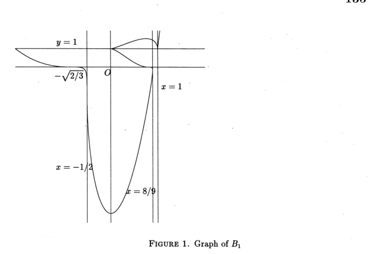
FIGURE 1. Graph of $B_{1}$
The purpose of this section is to construct another projective curve $C_{3}$ of degree 12 with 27
cusps such that $\pi_{1}(\mathrm{P}^{2}-C_{3})$ is abelian. The triple $\{C_{1}, C_{2}, c_{3}\}$ gives the first example of a
triple of projectivecurves whose $\mathrm{c}\mathrm{o}\mathrm{m}\mathrm{p}.1\mathrm{e}\mathrm{m}\mathrm{e}\mathrm{n}\mathrm{t}_{\mathrm{S}}$are topologically different. Therefore the moduli
space of curves of degree 12 with 27 cusps has at least 3 irreducible components.
We start with the following family of affine curves $B_{1}(t)$ of type (1,2;6) which is defined by
$B_{1}(t):=\{(x, y)\in \mathrm{C}^{2}; f_{t}(X, y)=0\},$ $t\in$ R. In [26], we have used this family to construct a
non-conical six cuspidal sextic where:
(5.1) $f_{t}(x, y)$ $:=x^{2}(x-1)^{2}(X2+2x+a_{00})+x(x-1)(a_{1}2X^{2}+a_{11}x+a_{10})(y-1)$
$+(a_{22}x^{2}+a_{21}x+a_{20})(y-1)^{2}+a_{30}(y-1)^{3}$
where $h=1-3t+3t^{2}$ and
$\{$
$a00=-(3t-2)^{2}/h$, $a_{12}=(-7+24t-27t^{2}+9t^{3})/h$, $a_{11}=3(1-2t-t2+3t^{3})/h$,
$a_{10}=4-6t$, $a_{22}=3t^{2}-9t+5$, $a_{21}=-4+6t$, $a_{20}=-h$, $a_{30}=(t-1)^{3}$
Note that $B_{1}(t)$ has two cusps at $(1,1)$, $(0,1)$ and twoflexes of order 1 at $(\pm\sqrt{t}, 0)$ with thesame
tangent line $y=0$. The pull-back by the flex double covering $\varphi$
:
$\mathrm{C}^{2}arrow \mathrm{C}^{2},$ $\varphi(x, y)=(x, y^{2})$
gives a family of six cuspidal sextics $B_{2}(t)$ which is defined by the polynomial $\hat{f}_{t}(X, y)$ $:=$
$f_{t}(x, y^{2})$. We will study the fiber $B_{1}(2/3)$ and $B_{2}(2/3)$ in detail, as they are ofspecial interest.
They are defined by the polynomials:
(5.2) $f_{2/3}(x, y)=x(2x-1)^{2}((X+1)^{2}-y)+(_{X^{2}}-1)(y-1)^{2}/3-(y-1)^{3}/27$
(5.3) $\hat{f}_{2/3}(x, y)=x^{2}(x-1)2((X+1)^{2}-y^{2})+(x^{2}-1)(y^{2}-1)^{2}/3-(y^{2}-1)3/27$
This family ofcurves enjoys the following properties.
(a) The polynomials$f_{t}$ and$\hat{f}_{t}$ are generic at infinity
for
$t\neq 2/3$ but $f_{2/3}$ and$\hat{f}_{2/3}$ are degeneratedHowever the curve $B_{2}(2/3)$ has no singularity at infinity but it has two
flex
points at infinity $[1; \pm\sqrt{3};0]$ with their common tangent line $L_{\infty}:=\{Z=0\}$.
(b) For each $t,$ $B_{1}(t)$ has two cusps at $S_{1}:=(1,1)$ and $S_{2}:=(0,1)$
.
The tangent cone at $S_{1}$ isconstant and it is
defined
by $x^{2}=0$. The tangent cone at $S_{2}$ is not constant. For $B_{1}(2/3)$, itis given by $y^{2}=0$
.
(c) The discriminant $\Delta_{y}(f_{2/3})(x)$ is given by
(5.4) $\Delta_{y}(f)(x)=x^{3}(-8+9x)(2x+1)^{2}(x-1)4$
and $\deg_{\dot{x}}(\Delta(yf2/3))=10$ and $\deg_{x}(\Delta_{y}(f_{t}))=12$
for
$t\neq 2/3$.
(Two rootsof
$\triangle_{y}(f_{t})(x)=0$disappear at infinity when $tarrow 2/3.$) $x=0$ and$x=1$ are roots
of
$\Delta_{y}(f_{t})(x)=0$of
multiplicity3 and 4 respectively and
$(\star)$
:
other rootsof
$\Delta_{y}(f_{t})(x)=0$ are simplefor
a generic $t$.For the last assertion $(\star)$, by the algebraicity of thecondition, it is enough to giveonegeneric
$t$ such that this is the case. For example, $\triangle_{y}(f_{3/4})(X)$ is given by
$-x^{3}(5504X4704x-2204\mathrm{s}_{-1}48X^{3}+81816x-5712X-401321)(x-1)^{4}/87808$
(d) The discriminant
of
$\hat{f}$ is given by ??and the equality $f_{2/3}(x, 0)=(3x^{2}-2)^{3}/27$, as
(5.5) $\Delta_{y}(\hat{f}_{2/3})(x)=cx^{6}(-8+9x)^{2}(2X+1)^{4}(x-1)^{8}(3_{X^{2}}-2)^{3}$
(e) $(-1/2, -5/4)$ is a
flex of
order1of
$B_{1}(2/3)$ whose tangent line is the vertical line $x=-1/2$.Thus $C^{a}(\hat{f}_{2/3})$ has two
flexes
at $(-1/2, \pm\sqrt{5}i/2)$ with the common tangent line $x=-1/2$.We have seen in section 3 that a smooth point $P\in C^{a}(f)$ is a flex point of order 1 if and
only if$d^{2}y/dx^{2}$ vanishes at $P$. As $dy/dx=- \frac{\partial f}{\theta x}/\frac{\partial f}{\partial y}$, this is equivalent to $\mathcal{F}(f)(P)=0$ where
$\mathcal{F}(f):=\frac{\partial^{2}f}{\partial x^{2}}(\frac{\partial f}{\partial y})^{2}-2\frac{\partial^{2}f}{\partial x\partial y}\frac{\partial f}{\partial x}\frac{\partial f}{\partial y}+\frac{\partial^{2}f}{\partial y^{2}}(\frac{\partial f}{\partial x}$
.
$)^{2}$
Using the algebraicity of this condition and the information from the real graph of $B_{1}(t)$ and
$B_{2}(t)$ for $|t-2/3|\leq\epsilon$ with $\epsilon$ sufficiently small, we can show that
(f) there exists a family
offlexes
$(\alpha(t), \beta(t))$of
$B_{1}(t)for|t-2/3|\leq\epsilon$ ($\epsilon$: sufficiently small) suchthat $(\alpha(2/3), \beta(2/3))=(-1/2, -5/4)$
.
Similarly there exists twofamilies of
flexes
$(\gamma(t), \pm\delta(t)i)$of
$B_{2}(t)$ such that $(\gamma(2/3), \delta(2/3)i)=(-1/2, \sqrt{5}i/2)$.
For example, $F(f_{2/3})(0, -8)>0$ and $\mathcal{F}(f_{2/3})(-3/4, b)<0$ where $b$ is the real solution of
$f_{2/3}(-3/4, b)=0$. For the existence of flexes for $B_{2}(t)$, we consider the graph of the real curve
$C^{a}(f’)$ with $f’(x, y, t):=f(x, iy, t)$. Then $(\gamma(t), \pm\delta(t))$ are real flexes of $C^{a}(f’)$. For later
purpose, we put $A_{\pm}(t)=(\gamma(t), \pm\delta(t)i)$. Note that $\gamma(t)\neq\alpha(t)$ for $t\neq 2/3$. $\alpha(t),$ $\beta(t),$$\gamma(t)$ and $\delta(t)$ are real numbers and wemay assume $\delta(t)>0$.
(g) The tangent lines at $A_{+}(t)$ and $A_{-}(t)$ are not vertical
for
$t\neq 2/3$.Note that the inverse image of a flex point of$B_{1}(t)$ is not a flex of$B_{2}(t)$ if the tangent line of
a flex is not vertical. Here “vertical” implies $\partial f/\partial y$vanishes. In fact, assume that $\gamma(t)=\alpha(t)$
and the tangent line at $(\alpha(t), \beta(t))$ is vertical. This implies that $\triangle_{y}(f_{t}, y)(x)$ has the factor
5.2. Recipe of the construction of a
curve
$C_{3}$.
The generic $(2,2)$-fold cyclic covering$C_{2,2}(B_{2}(t))$ of $B_{2}(t)$ gives a curve of degree 12 with 24 cusps with $\pi_{1}(\mathrm{P}^{2}-C_{2,2}(B_{2}(t)))\cong$
$\mathrm{Z}_{12}$. See [28]. It is the purpose of this section to put three more cusps without breaking the
commutativity of the fundamentalgroup. We first take the double covering along the tangent
line at the flex $A_{-}(t)$ and we denote the pull-back of $B_{2}(t)$ by $B_{3}(t)$
.
We have seen that thetangent lines at $A_{\pm}(t)$ degenerate at $t=2/3$ into the same line $x=-1/2$. Thus $B_{3}(t)$ has
13 cusps for $t\neq 2/3$ and 14 cusps for $t=2/3$
.
Let $g_{t}(x, y)$ be the defining polynomial of$B_{3}(t)$. Though $\pi_{1}(\mathrm{C}^{2}-B_{3}(2/3))$ may benot abelian, wecan show, using the geometry of this
degeneration, that $\pi_{1}(\mathrm{C}^{2}-B3(t))$ is abelian for any $t$, provided $|t-2/3|$ is sufficiently small
and $t\neq 2/3$ (thus abelian for any generic $t$). We will see that flex curves of $B_{3}(2/3)$ disappear
at infinity. Finally we take a generic
flex
double covering$\mathcal{F}^{(2)}(gt;P)$ which is a curve of degree12 with
27
cusps and we put $C_{3}:=\mathcal{F}^{(2)}(g_{t;}P)$. We will refer the detail of the proof to [30].6. $\mathrm{A}_{\mathrm{L}\mathrm{E}\mathrm{x}}\mathrm{A}\mathrm{N}\mathrm{D}\mathrm{E}\mathrm{R}$
POLYNOMIAL
6.1. Alexander polynomial through Fox calculus. We quickly recall the definition of
Alexander polynomial of a finitely representable group $G$ with a surjective homomorphism
$\varphi$ : $Garrow \mathrm{Z}$. Let $F_{n}$ be a free group with $n$-generators $X_{1},$
$\ldots$ ,$X_{n}$ and let $G$ be a finitely
represented group with $n$-generators $x_{1},$ $\ldots$,$x_{n}$ and assume that the kernel of the surjective
map $\psi$ : $F_{n}arrow G$, defined by$\psi(x_{i})=x_{i}$, is normally generated by $R_{1},$
$\ldots,$$R_{s}\in F_{n}$. Let $C[F_{n}]$,
$\mathrm{C}[G]$ and $\mathrm{C}[\mathrm{Z}]$ be the respective group rings of $F_{n},$ $G$ and $\mathrm{Z}$ with $\mathrm{C}$ coefficients. We can
identify $\mathrm{C}[\mathrm{Z}]$ with the Laurent polynomial ring $\mathrm{C}[t, t^{-1}]$, under a fixed generator$t\in \mathrm{Z}$. There
are canonical homomorphisms $\psi_{*}:$ $C[F]narrow \mathrm{C}[G]$ and $\varphi_{*}:$ $\mathrm{C}[c]arrow \mathrm{C}[t,t^{-1}]$ which are induced
by $\psi$ and
$\varphi$. The j-th Fox derivative $\partial/\partial X_{j}$ is a linear map $\mathrm{C}[F_{n}]arrow \mathrm{C}[F_{n}]$, characterized by
the following properties:
$\frac{\partial X_{i}}{\partial X_{j}}=\delta_{ij}$, $\frac{\partial uv}{\partial X_{j}}=\frac{\partial u}{\partial X_{j}}+u\frac{\partial v}{\partial X_{j}}$, $u,$$v\in \mathrm{C}[F_{n}]$
To $(G, \psi, \varphi)$, we associate $s\cross n$-matrix $M$ of$\mathrm{C}[t, t^{-1}]$ coefficients whose $(i, j)$-entry is given by
$a_{ij}:= \varphi_{*}(\psi_{*}(\frac{\partial R}{\partial X_{j}}))$. The Alexander polynomialof $G$ with respect to $\varphi$ : $Garrow \mathrm{Z}$ is defined by
the greatest common divisor of $(n-1)\cross(n-1)$-minors of $M$. This does not depend on the
choice of the representation $\psi$ and the choice of generators $R_{1},$
$\ldots,$$R_{\epsilon}$ of the kernel. See [8] and
[21] for further detail.
Let $C$ be an irreducible affine curve of degree $d$. Then weknow that $H_{1}(\mathrm{C}^{2}-c;\mathrm{z})\cong \mathrm{Z}$ and
the Hurewicz homomorphism together with this identification gives a surjective homomorphism
$\xi$ : $\pi_{1}(\mathrm{C}^{2}-C)arrow H_{1}(\mathrm{c}^{2}-c;\mathrm{z})\cong \mathrm{z}$
We fix a generator $t\in H_{1}(\mathrm{C}^{2}-\mathit{0};\mathrm{z})$ so that any lasso $\tau\in\pi_{1}(\mathrm{C}^{2}-C)$ for $C$ corresponds to
$t$ through the Hurewicz homomorphism. The Alexander polynomial of$C$ is defined by that of
$\pi_{1}(\mathrm{C}^{2}-C)$ with respect to the Hurewicz homomorphism $\xi$ and we denote it by $A_{C}(t)$.
Example 6.1. 1. Let $C$ be an irreducible affine curve with an abelian fundamental group.
Then we can use the trivial representation $\psi=\mathrm{i}\mathrm{d}:F_{1}arrow \mathrm{Z}$. Thus $A_{C}(t)=\dot{1}$.
2. Let $Z_{6}$ be asix cuspidal conical sextic with respect to a generic line at infinity (see [Z1]).
Then the fundamental group $\pi_{1}(\mathrm{C}^{2}-Z_{6})$ has the representation $\langle x,y;Xyx=yxy\rangle$ (see for
example [26]$)$
.
As the generators$x,$$y$ are lassos for $Z_{6}$, they corresponds to $t$ via Hurewicz
homomorphism. We can take $s=1,$ $R_{1}=X\mathrm{Y}X\mathrm{Y}^{-1}X-1\mathrm{Y}^{-1}$ . Then $\partial R_{1}/\partial X$ and $\partial R_{1}/\partial \mathrm{Y}$ $\mathrm{g}\mathrm{i}\mathrm{v}\mathrm{e}\pm(t^{2}-t+1)$ respectively. Thus $A_{Z_{6}}(t)=t^{2}-t+1$
.
3. Let $Z_{4}$ be the three cuspidal quartic with respect to a generic line at infinity. Then
$R_{2}=x^{2}y^{-2}$
.
Then $\partial R_{1}/\partial X$ and $\partial R_{1}/\partial \mathrm{Y}$ give the same polynomial $t^{2}-t+1$.
$\partial R_{2}/\partial X$ and $\partial R_{2}/\partial \mathrm{Y}$ give the linear $\mathrm{f}\mathrm{o}\mathrm{r}\mathrm{m}\pm(t+1)$. Thus we have$A_{Z_{4}}(t)=1$.
The following is an immediate consequence of Lemma 2.1.
Lemma 6.2. Let $f(x, y)$ be a $wt$-convenient polynomial
of
type $(a, b;d)$ and let $D=\{y=0\}$and $f_{m}(x, y):=f(x, y^{m})$. Let $\iota_{1}$ : $\mathrm{C}^{2}-c^{a}(f)\cup Darrow \mathrm{C}^{2}-c^{a}(f)$ and $\iota_{2}$ : $\mathrm{C}^{2}-c^{a}(f)\cup Darrow$
$\mathrm{C}^{2}-D$ be the respectiv’e inclusion map and assume
that the canonical homomorphism
$\iota_{1\#}\cross\iota_{2\#}$
:
$\pi_{1}(\mathrm{C}^{2}-ca(f)\cup D)arrow\pi_{1}(\mathrm{C}^{2}-^{c}a(f))\mathrm{x}\pi_{1}(\mathrm{C}^{2}-D)$is isomorphism. Then the Alexander polynomial
of
$C^{a}(f_{m})$ is equal to thatof
$C^{a}(f)$.
Applying this lemma to the generic $(3,3)$-covering transform $C_{1}:=C_{3,3}(Z_{4})$ of the Zariski’s
three cuspidal quartic $Z_{4}$ and the curve $C_{3}$ which we have constructed in the section 5, we
obtain:
Corollary 6.3. The Alexander polynomials
of
$C_{1}$ and $C_{3}$ coincide.Such a pair of non-irreducible plane curves are known by [3]
REFERENCES
[1] N. A’Campo and M. Oka, Geometry ofplane curves via Tschirnhausen resolution tower, Osaka J. Math., vol. 33,no. 4 (1997), 1003-1034.
[2] E. Artal, Surles couples des Zariski, J.Algebraic Geometry,vol3 (1994), 223-247.
[3] E. Artal andJ. CarmonaZariskipairs,fundamentalgroups andAlexander polynomials, preprint, 1995
[4] E. Artin, Theory ofbraids,Ann. of Math., vol48 (1947), 101-126.
[5] D.N. Bernshtein, The number of roots of a system of equations, Funktsional’nyi Analiz i Ego Prilozheniya, vol9 (1975), 183-185.
[6] E. Brieskorn and H. Kn\"orrer, Ebene Algebmische Kurven, Birkh\"auser(1981), Basel-Boston- Stuttgart.
[7] D. Cheniot, Le groupe
fondamental
du compl\’ementaire d’une courbe projective complexe, Ast\’erique, vol7 et 8 (1973), 241-253.
[8] R.H. Crowell and R.H. Fox, Introduction to Knot Theory, Ginn and Co. (1963).
[9] P. Deligne, Le groupe fondamental du compl\’ement d’une courbe plane n’ayant que des points doubles ordinaires est ab\’elien, S\’eminaire Bourbaki (1979/80), vol no. 543.
[10] I. Dolgachev and A. Libgober, On thefundamentalgroup ofthe complement to a discriminantvariety,
in: Algebraic Geometry,Lecture Note 862 (1980), 1-25, Springer, Berlin Heidelberg New York.
[11] R. Ephraim, Special polars and curves with one place at infinity, in: Proceeding of Symposia in Pure Mathematics, 40,AMS (1983), 353-359.
[12] W. Fulton, On the
fundamental.group
ofthe complement of a node curve, Annals of Math.,vol111 (1980), 407-409.[13] P. Griffiths and J. Harris, Principles ofAlgebraic Geometry, 1978 A Wiley-Interscience Publication, New$\mathrm{Y}\mathrm{o}\mathrm{r}\mathrm{k}-\mathrm{c}\mathrm{h}\mathrm{i}\mathrm{C}\mathrm{h}\mathrm{e}\mathrm{s}\mathrm{t}\mathrm{e}\Gamma^{-\mathrm{B}\mathrm{i}\mathrm{s}}\mathrm{r}\mathrm{b}\mathrm{a}\mathrm{n}\mathrm{e}$-Toronto.
[14] R.C. Gunningand H. Rossi, Analytic
functions
ofseveral complex variables, 1965,Prentice-Hall, London[15] H.W.E. Jung, \"Uber ganze birationale hansfomationen der Ebene, J. Reine Angew. Math., vol184
(1942), 1-15.
[16] E.R. van Kampen, On the fundamental group ofan algebraic curve, Amer. J. Math., vol55 (1933),
255-260.
[17] S. Lang, Algebra, Addison-WesleyPub., 1965.
[18] D.T. L\^e and M. Oka, On resolution complexity ofplane curves,Kodai Math. J., 1-36, Vol. 18, 1995
[19] V.T. Le and M. Oka, Estimation of the Number of the Critical Values at Infinity of a Polynomial
Function$f:\mathrm{C}^{2}arrow \mathrm{C}$, Publ. RIMS, Kyoto Univ., vol. 31, no. 4 (1995), 577-598.
[20] D.T. L\^e and C.P. Ramanujam, The invariance ofMilnor’s number implies the invariance ofthe
topo-logical type,Amer. J. Math., vol. 98, no. 1 (1973),67-78.
[21] A. Libgober, Alexanderpolynomialofplane algebraic curves and cyclic multiple planes, Duke Math. J., vol. 49,no. 4 (1982),833-851.
[22] J. Milnor, Singular Points of Complex Hypersurface, Annals Math. Studies, vol61 (1968), Princeton
[23] M. Oka, On thefundamentalgroupofa reducible curve in$\mathrm{P}^{2}$, J. London
Math. Soc. (2), vo112(1976),
239-252.
[24] M. Oka, Someplanecumes whose complements havenon-abelianfundamentalgroups, Math. Ann.,vol
218 (1975),55-65.
[25] M. Oka, On the
fundamental
groupof
the complementof
certainplane curves, J.Math. Soc. Japan,vol30 (1978), 579-597.
[26] M. Oka, $symmet7\dot{\mathrm{Y}}C$ plane cumes with nodes and cusps, J. Math. Soc. Japan,
vol44, no. 3 (1992),
375-414.
[27] M. Oka, Geometry ofplane curves via toroidal resolution,in: Singularities and Algebraic Geometry,
1995, Birkh\"auser, Basel,95-121.
[28] M. Oka, Two $t\dot{r}anSfomS$ ofplane curves and theirfundamentalgroups,J. Math. Sci. Univ.
Tokyo, vol
3 (1996), 399-443.
[29] M. Oka, Moduli space ofsmooth affine curves ofa givengenus with oneplace at infinity, to appear.
[30] M. Oka, Flexcurves and their applications, preprint 1997
[31] M. OkaandK.Sakamoto, Producttheoremofthefundamentalgroupofa reducible curve,J. Math.Soc.
Japan, vol30,no. 4 (1978), 599-602.
[32] D.W. Sumners, On the homology of
finite
cyclic coverings ofhigher-dimensional links, Proc. Amer.Math. Soc. vol46 (1974), 143-149.
[33] O. Zariski, Onthe problem ofexistenceofalgebraicfunctions
of
twova$r\dot{?}ables$possessinga given branchcurve, Amer.J. Math. vol51 (1929), 305-328.
[34] O. Zariski, On the Poincar\’egroup ofrationalplanecurvesAmer. J. Math. vol58 (1929), 607-619.
[35] O. Zariski, On the Poincar\’egroup ofaprojective hypersurface,Ann. of Math.,vol38 (1937), 131-141.
DEPARTMENT OF MATHEMATICS, TOKYO METROPOLITAN UNIVERSITY
$\mathrm{M}\mathrm{l}\mathrm{N}\mathrm{A}\mathrm{M}1$-OHSAWA,
HACHIOJI-SHI TOKYO 192-03, JAPAN
$E$-mailaddress: $\mathrm{o}\mathrm{k}\mathrm{a}\emptyset \mathrm{m}\mathrm{a}\mathrm{t}\mathrm{h}$.metro-u. $\mathrm{a}\mathrm{c}$