Gravity Waves Observed in a High-Resolution GCM Simulation(Pattern Formation and Singularity in Wave Phenomena)

Gravity Waves Observed

in

a

High-Resolution

GCM

Simulation

By

Kaoru Sato

Department of Geophysics, Faculty ofScience, _KyotoUniversity ToshiroKumakura

Department of CiviI andEnvironmentalEngineering, Nagaoka University of Technology and

Masaaki Takahashi

Center for ClimateSystemResearch,University of Tokyo

1

Introduction

Alot ofefforts havebeenmade toelucidategravity

wave

characteristics in the real atmosphere using various observational data. However,observational stations

are

notuniformly distributed

on

the earth and usually

we

cannotobtain all physical quantities from observations which

are

needed forthe analysis. Thus,

we use a

GCM with high resolution both in the horizontal and vertical directionstoexamine global characteristics ofgravity

waves

in the lower stratosphere.

2

Model Experiments

Themodel usedis the first version of the atmospheric general circulation model (GCM)which

was

developedatthe Center forClimateSystem$\mathrm{R}\mathrm{e}\mathrm{s}\mathrm{e}\mathrm{a}\mathrm{r}\mathrm{c}\mathrm{h}/\mathrm{N}\mathrm{a}\mathrm{t}\mathrm{i}_{0}\mathrm{n}\mathrm{a}1$Institute for Environmental

Studies $(\mathrm{C}\mathrm{C}\mathrm{S}\mathrm{R}/\mathrm{N}\mathrm{I}\mathrm{E}\mathrm{S})$ (Numaguti, 1993; Numaguti etal., 1995; Nakajimaet al. (1995). The

horizontalresolution isT106, whichcorrespondsto

a

gridspacingof about120km. There

are

53

layers inthe vertical,havingabout600$\mathrm{m}$vertical resolution in theuppertroposphere and lower

stratosphere. This fine vertical gridspacingisnecessarytoresolvesmall vertical wavelengths of gravity

waves as

observed in the real atmosphere. The top level of the model is locatedatabout

0.5

$\mathrm{h}\mathrm{P}\mathrm{a}$. The moist convective adjustment scheme is used

as

the cumulus parameterization

in this experiment following Takahashi (1996) who successfully obtained realistic QBO in

a

GCM.Thebottom boundary condition is that of

an

aqua-planet. Values of SST climatology in February

are

given independent of longitude and time(perpetual February). The otherprocesses

andschemes

are

almost the

same as

thoseinthestandard GCMexperiments. As for thestart-up

lun,

a

horizontal resolution T21,

53

layers $(\mathrm{T}21\mathrm{L}53)$ model of the

same

boundary condition

was

integrated with

an

initial condition of

an

isothermal atmosphere at rest

over

120 model daysto obtain

a

quasi-steady state. Thefinal day of$\mathrm{T}21\mathrm{L}53$ model simulation

was

used

as

the

initial condition of the$\mathrm{T}\mathrm{l}06\mathrm{L}53$ model. The$\mathrm{T}\mathrm{l}06\mathrm{L}53$ model

was

run

for

80

days and obtained

a

quasi-steady state. The data of final 20 days at

a

time interval of 1 hour

were

used forthe analysis of gravity

wave

activities. To avoid aliasing from fluctuationswithhigher frequencies, values averaged

over one

hour

are

used. As

a

result

we

obtained

a

realistic

mean

zonal wind

field. The$\mathrm{s}\mathrm{u}\mathrm{b}\mathrm{t}\mathrm{r}_{1}\mathrm{o}-\mathrm{p}\mathrm{i}_{\mathrm{C}}\mathrm{a}1$ westerlyjet is situated around

$32\mathrm{N}$and$45\mathrm{S}$,withpeak values larger than

40and30$\mathrm{m}\mathrm{s}$ ,respectively. The polar nightjet and subtropicaljet

are

clearly separated in the

northernhemisphere. The tropopause heights

are

alsorealistic;

15-16

kmin the tropicalregion

and about9-10kmin the middle and high-latitude regions.

3

Comparison With

MST

Radar

Observations

To

see

how realistic the gravity

wave

field simulated in this model is,

we

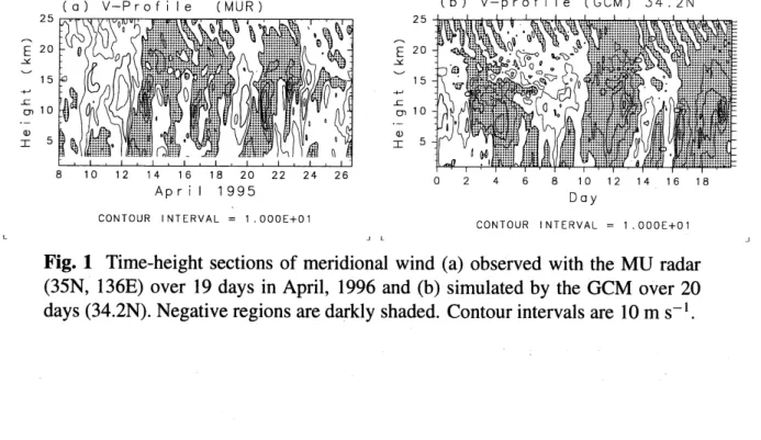
made comparison

with observation data. Figure lashows

a

time-height sectionof meridional winds (v) obtained through

a

special long-term(19days)continuous observation with the MU (Middle_{and Upper}

atmosphere)radarwhichis

an

MST radarlocatedatShigaraki, Japan$(35\mathrm{N}, 136\mathrm{E})$

.

See Fukaoet $\mathrm{a}1.(1985)$for details of the MU radar. Clear downwardpropagatingphasestructureisobserved

in the heightregionof

19-25

km(seecontoursof$0$

or

10$\mathrm{m}\mathrm{s}^{-1}$),where the zonal

mean

windis

very weak. Thevertical wavelength and

wave

period

are

about

3.5

km and 20$\mathrm{h}$,

respectively. Satoetal. (1997) made detailedanalysis and showed that the

wave

structure is due to inertia-gravity

waves

with

a

horizontal wavelength of about 1200 km propagating westward with

a

phase speed of about 10$\mathrm{m}\mathrm{s}^{-1}$. The vertical and horizontal wavelengths

are

sufficiently large tobe resolvedin

our

high-resolution model.

Figure lb shows

a

time-heightsection of simulated$v$ atthelatitude of34.$2\mathrm{N}$

over

20days.

The tickmarks

on

theright indicate the locations of vertical grids in the model. The tilt of

zero

contours of the simulated $v$ (e.g., Day 10 and Day 16) is similarto that ofradar observation

(e.g., 12 and20April), indicating that simulated baroclinic

waves

are

realistic. Mostimportant

is the feature that gravity

wave

structure having vertical wavelength and

wave

period similar to observation is

seen

in lower stratosphere in the model data. Comparison ofpowerspectra indicates that the amplitude of simulated gravity

waves

accords with observation. This good

$\mathrm{a}\mathrm{g}\mathrm{r}\mathrm{e}\mathrm{e}\mathrm{m}\mathrm{e}\ulcorner \mathrm{n}\mathrm{t}$ withobservationssuggeststhat the

$\mathrm{g}\mathrm{r}\mathrm{a}\urcorner\ulcorner$vity

wave

field in

our

modelis fairly realistic. $\neg$

CONTOUR }$\mathrm{N}\mathrm{T}\mathrm{E}$RVA$\llcorner$ $=$ 1 000$\mathrm{E}+01$

CONTOUR I$\mathrm{N}\mathrm{T}\mathrm{E}$RVA$\mathrm{L}$ $=$ 1 000$\mathrm{E}+01$

Fig. 1 Time-height sections of meridional wind (a) observed with the MU radar

$(35\mathrm{N}, 136\mathrm{E})$

over 19

days in April,

1996

and (b) simulatedby the GCM

over

20

4 Stati

$s$

tical

Characteristics

of

Gravity Waves

Since there is

no

_{longitudinal dependence of boundary condition inthe presentmodel,the}

statis-tical characteristicsofgravity

waves

mustbe independent of longitude. Thus, inthe following

sections

we

analyzetime seriesofeight longitudes with the

same

longitudinalinterval$(45^{\mathrm{o}})$ and

examinethe

average as

thestatisticsof the model.

4.1

Spectral

characteristics

as a

function

of latitude

Frequencypowerspectra

were

calculatedateach of eight longitudes

as

a

function of latitude$(\phi)$

andheight$(z)$, andthe

average

ofeightspectra

was

obtained. The spectra

were

_{further averaged}

for the the heightregionsof

22-27

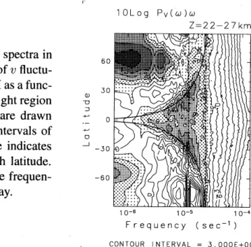
km with fine vertical resolution. Aresultfor$v$ is shown in

Fig. 2. Thick solid

curves

indicate the inertial frequencyateach latitude and red dashed

curves

indicate the periods of

one

day and

a

half day.

Large values

are

distributed at higher frequency regions bordered with the

curve

of the inertial frequency. This is consistentwith the theory of internal gravity

waves

that their

wave

frequencies should be higher than the inertial frequency. An interesting featureis that isolated peaks

are

observed around the inertial frequencyateach latitudeexceptaround theequator. The spectra aroundtheequatorwhere the inertial frequency becomes

zero

are

widely distributed and

no

particular peaks

are

observed.

Fig. 2 Frequency

power

spectra in theenergy-contentformof$v$

fluctu-ationssimulated by GCM

as a

func-tionoflatitude for the height region of $22-27\mathrm{k}\mathrm{m}$

.

Contours

are

drawn

for $10\log P(v\omega)\omega$ with intervals of

$3\mathrm{d}\mathrm{B}$

.

A thick solid

curve

indicates

inertial frequency at each latitude. Two dashed lines indicate frequen-cies of 1 day and

a

half day.

$\mathrm{F}\ulcorner \mathrm{e}\mathrm{q}_{\mathrm{U}\mathrm{e}}\mathrm{n}\mathrm{c}\mathrm{y}$ $(\mathrm{s}\mathrm{e}\mathrm{c}-))$

CON$\mathrm{T}$OU$\mathrm{R}$ I$\mathrm{N}\mathrm{T}\mathrm{E}\mathrm{R}$VA$\mathrm{L}$ $=$ $3$ $000\mathrm{E}+\mathrm{o}\mathrm{o}$

4.2

$\mathrm{G}\mathrm{l}\mathrm{o}\mathrm{b}\mathrm{a}\mathrm{l}\mathrm{e}\mathrm{n}\mathrm{e}\mathrm{r}\mathrm{g}\mathrm{y}\mathrm{d}\mathrm{i}S\mathrm{t}\Gamma \mathrm{i}\mathrm{b}\mathrm{u}\mathrm{t}\mathrm{i}\mathrm{o}\mathrm{n}\mathrm{a}\mathrm{n}\mathrm{d}\mathrm{m}\mathrm{e}\mathrm{r}\mathrm{i}\mathrm{d}\mathrm{i}_{\mathrm{o}\mathrm{n}}\mathrm{a}\mathrm{l}\mathrm{P}\Gamma \mathrm{o}\mathrm{p}\mathrm{a}\mathrm{g}\mathrm{a}\mathrm{t}\mathrm{i}\mathrm{o}\mathrm{n}\mathrm{o}\mathrm{f}\mathrm{g}\mathrm{r}\mathrm{a}\mathrm{v}\mathrm{i}\mathrm{t}\mathrm{y}_{\mathrm{W}}\mathrm{a}\mathrm{V}\mathrm{e}s$

We made

energy

and momentum flux analysis for two kinds ofcomponents, which

are

fre-quently treated

as

gravity

waves

in observational studies: short-period ($<1$ day)

waves

and

horizontal propagation of intemal gravity

waves.

Positive (negative) eastward

(westward) propagation and positive (negative) $\overline{\prime\prime}$$vw$

means

northward (southward)

propaga-tion relative to the

mean

wind for gravity

waves

propagating

energy

upward. The signs

are

reversed for downward

energy

propagation. The vertical

energy

flux$\overline{p’w’}$, where

$p$ isthe

pres-sure,indicates dominance of upwardenergy propagationin the lower stratosphere for bothtwo kinds ofgravity

wave

components.

The distribution $\mathrm{o}\mathrm{f}\overline{u’w’}$showstheshort-period gravity

waves

propagate westward relative

to the

mean

wind (not shown). Interesting

are

the characteristics $\mathrm{o}\mathrm{f}\overline{v^{\prime/}w}(\mathrm{F}\mathrm{i}\mathrm{g}.3\mathrm{a})$

.

Negative

(positive)values

are

observed in the southern(northern) hemisphere. Moreoverthe latitudinal

expanse

oflarge$vw$$\overline{\prime l}$i

sncrease as

altitude increases. The edge of the large$\overline{v^{\prime_{w’}}}$regionreaches

themid-latitude of$\phi=50^{0}\mathrm{a}\iota Z=27$km. This$\mathrm{V}$-shaped distribution suggeststhatgravity

waves

are

generated in the equatorialregion andpropagate poleward in both hemispheres.

The

energy

andmomentumflux features of small vertical-scale

waves are

similarto those

of short period

waves: wave

energy is maximized around the equator; the

waves

propagate westward relative to the

mean

wind. Howeverthere

are a

few remarkable differences. Figure

$3\mathrm{b}$shows latitude-height sections$\mathrm{o}\mathrm{f}\overline{v’ w’}$for small vertical-scale

waves.

Itis noted that negative

(positive) values $\mathrm{o}\mathrm{f}\overline{v’ w^{J}}$above thesubtropical jet in the northem (southem) hemisphere. This

means

equatorward propagation ofgravity

waves

and is consistent with observations (Sato,

1994). This feature isnot

seen

for short-period

waves.

Thus small vertical-scale

waves

prop-agating equatorward above the subtropical jethave

wave

periods longerthan 1 day. The$\overline{v’w’}$

profile in the equatorial region suggests the dominance of polewardpropagationfrom the

equa-tor,similarto short-periodwaves,but themagnitude is smaller. Thusshort-period

waves

prop-agatingpoleward have vertical wavelengths longer than5 km.

A westwardforcecalculatedfrom theEliassen-Palmflux due togravity

waves was

5$\mathrm{m}\mathrm{s}^{-11}\mathrm{m}\mathrm{o}\mathrm{n}\mathrm{t}\mathrm{h}^{-}$

atthemaximum in the

upper

part ofthesubtropical westerly jetaround $30\mathrm{N}$, whichis smaller

by

one

order of magnitude compared with the drag duetotopographically forced gravity

waves

(e.g. Palmeretal., 1986; $\mathrm{M}\mathrm{c}\mathrm{F}\mathrm{a}\mathrm{r}\mathrm{l}\mathrm{a}\mathrm{n}\mathrm{e}$, 1987).

5

Concluding

Remark

$s$

With the aid of

a

high-resolution GCM $(\mathrm{T}106\mathrm{L}53)$, global distribution and characteristics of

gravity

waves were

examined. By using subsets outofthe huge amount of data obtained with this high-resolution GCM simulation like observational data, further interesting analyses are

possible: three dimensional structure of gravity

waves

having near-inertial frequency in the stratosphere; the generation and interaction with synoptic-scale baroclinic

waves

of gravity

waves

thatare dominant above thesubtropical jet; and thepossible role of small-scalegravity

waves on

the QBO in the equatorial stratosphere. However, it is

a

matter of course, and

we

CONTOUR I NT$\mathrm{E}$RVA$\mathrm{L}$ $=$ $2$ 000 E-03 CON$\mathrm{T}$OUR I NT$\mathrm{E}$RVA$\mathrm{L}$ $=$ $2$ 000 E-03

Fig.

3

Latitude-height sections of vertical fluxes of meridionalmomentum$(v’w)\overline{/}$for

(a)short-periodgravity

waves

and(b)small vertical-scale

waves.

Contour intervals

are 0.002

$\mathrm{m}^{2}\mathrm{s}^{-2}$

.

Negative regions

are

shaded.

Acknowledgment

This study

was

supportedby Centerfor Climate System Research ofthe University of Tokyo, partly by

a

Grant-in-AidforScientific Research(A)(2)08404026 $(\mathrm{K}\mathrm{S})$and(B)

06452083

$(\mathrm{M}\mathrm{T})$

of the Ministry ofEducation, Science and Culture, Japan, and by Intemational Cooperative Study of Stratospheric Change and itsRolein ClimatefromtheScienceandTechnology Agency of Japan $(\mathrm{T}\mathrm{K})$. A part of calculation of the low resolution model

was

made by KDK (Kyoto

daigaku Denpakagaku Keisanki-jikken souchi) Radio Atmospheric Science Center (RASC)

of Kyoto University. The MU radar belongsto and is operated by RASC of Kyoto University. GFD-DENNOU library

were

used for drawing figures. This

paper

was submitted to J. Atmos. Sci.

REFERENCES

1. Fukao, S., T. Sato,T. Tsuda, S.Kato, K. Wakasugi and T.Makihira, 1985:RadioSci., 20,

1155-1168.

2. McFarlane, N.A., 1987: J. Atmos. Sci., 44,

1775-1880.

3. Nakajima, T., M. Tsukamoto, Y. Tsusima, and A. Numaguti,

1995:

Studies

_of

global environmentchange with special

_reference

toAsiaand

_Pacific

regions, I-3, 104-123. 4. Numaguti, A.,M. Takahashi,T. Nakajima, and A. Sumi,

1995:

ibid, I-3, 1-27.

5.

Numaguti,A.,

1993:

J. Atmos. Sci., 50,

1874-1887.

6.

Palmer, T.N., G.J. Shutts, and R. Swinbank,

1986:

Quart. J. Roy. Met. Soc., 112,

1001-1040.

7. Sato, K.,

1994:

J. Atmos. Terr. Phys., 56,

755-774.

8. Sato, K., D. J. O’Sullivan and T. J. Dunkerton, 1997: Geophys. Res. Lett., 24,

1739-1742.