An application of Draghicescu's fast summation method to vortex sheet motion

An

application

of

Draghicescu’s

fast

summation

method

to vortex

sheet

motion

Takashi

SAKAJO

and Hisashi

OKAMOTO

Research Institute for Mathematical

Sciences

Kyoto University, Kyoto,

606-01

Japan

September 2,

1996

Abstract

The fast summation method of Draghicescu is appliedto computationof$2\mathrm{D}$ vortex

sheet motions. In the present paper we report our numerical experimentswhich show

the effectiveness as well as difficulties of Draghicescu’s fast summation method in $2\mathrm{D}$

vortex-sheet computations. For instance, the fast summation method is nearly five

times faster than the direct summation method when we use 16,$384=2^{14}$ _vortex

blobs. On the other hand, if it is used together with the Fourier filter, the method is

found to be sensitive tothe filter threshold.

1

Introduction

We perform some numerical experiment on Draghicescu’s fast summation method. It is

appliedto acomputationof$2\mathrm{D}$ vortex sheetmotion. Ouraim is to compare the performance

of the fast summation with that of the direct summation.

What we consider is the Birkhoff-Rott equation with periodic boundary condition $($

Krasny $[6, 7])$. Namely,

we

consider the following equation:

$\frac{\partial z(t,\mathrm{r})*}{\partial t}=\frac{1}{2_{\dot{i}}}\mathrm{p}.\mathrm{v}.\int_{0}^{1}\cot\pi(Z(t, \mathrm{r})-z(t, \mathrm{r}’))d\Gamma’$ , (1)

where $t$ represents time, the integral is Cauchy’s principal value, $\dot{i}=\sqrt{-1},$ $\mathrm{a}\mathrm{n}\mathrm{d}*\mathrm{i}\mathrm{m}\mathrm{p}\mathrm{l}\mathrm{i}\mathrm{e}\mathrm{s}$ the

complex conjugate.

The vortex sheet is represented by the

curve

$z(t, \Gamma)=x(t, \Gamma)+\dot{i}y(t, \Gamma)$ with $\Gamma$ being

taken along the

curve.

$\Gamma$ is called the circulation parameter. The physical space is filled

with an inviscid incompressible fluid, whose motion is irrotational everywhere except on a

Birkhoff-Rott equation, see [6, 7, 9].

Krasny $[6, 7]$ solved (1) with Chorin’s vortex blob _{approximation and the Fourier filter.}

In the present paper,

we

add another technique, Draghicescu’s fast summation method, to

Krasny’s method. We then compare the performances. In the

course

of our study, we

found that Draghicescu’s method directly applied to the equation (1) has some difficulty in

programming. The difficulty, whichwe will explain in section 3, can be reduced ifwe put

$w=\exp(2_{T\dot{i}Z})$

and if (1) is rewritten as

$\frac{\partial w(t,\mathrm{r})^{*}}{\partial t}=-\pi\dot{i}w^{*}\mathrm{P}^{\mathrm{V}.\int_{0}^{1}}.\frac{w(\Gamma,t)+w(\Gamma/,t)}{w(\Gamma,t)-w(\mathrm{r}’,t)}d\Gamma’$. (2)

The

reason

why this equation has advantage

over

(1) will be given in section 3.

Thepresentpaper consists of five sections. In section 2, weexplainthe numerical method.

In section 3, wereport what we obtained in ournumerical experiments. Herewe focusonthe

computational $\mathrm{a}\mathrm{d}\mathrm{V}\mathrm{a}\mathrm{n}\mathrm{t}\mathrm{a}\mathrm{g}\mathrm{e}/\mathrm{d}\mathrm{i}_{\mathrm{S}}\mathrm{a}\mathrm{d}_{\mathrm{V}\mathrm{a}\mathrm{n}\mathrm{t}\mathrm{a}}\mathrm{g}\mathrm{e}$ of the method. Section 4 is devoted to

phenomeno-logical description of the sheet. The relation between the fast summation and Fourier filter

is discussed in section 5. Concluding remarks are presented in section 6.

2

$\delta$

Equation and

Discretization

In the computation, we use a smoothedversion of (2). Namely, wefollow Krasny’s idea ([7])

of desingularization. Specifically, we consider

$\frac{\partial w(t,\mathrm{r})^{*}}{\partial t}=\int_{0}^{1}K_{\delta}(w(t, \mathrm{r}),$ _{$w(t, \Gamma/))d\mathrm{r}’$}.

(3) where

$K_{\delta}(w, v)=- \pi iw\frac{(w+v)(w^{*}-v^{*})}{|w-v|^{2}+\delta^{2}}*$.

Note that the equation (3) reduces to (2) when $\delta=0$. We solve (3) with

some

initial

condition, $w(\mathrm{O}, \Gamma)$.

The equation (1) is known to be ill-posed (see, e.g., Caflisch et al. [1]). The smoothed

version (3) is, however, well-posed for any time interval if$\delta>0$. The high frequency modes

are

stabilized, see for instance [7].

We discretize (3) by the point vortices. Choosing a positive integer $N$, we consider the

following system of ordinary differential equations:

with the following initial condition:

$w_{n}(0)= \exp(\frac{2\pi\dot{i}n}{N}-\pi+2\pi i\epsilon(1-\dot{i})\sin(\frac{2\pi in}{N}))$ _{$(n=1,2, \cdots, N)$}. (5)

Here $\epsilon$ is a constant, which we fix to $\epsilon=0.01$.

This initial date is a rescaled function from

the one considered in Krasny [7]. The

reason

of rescaling is that after transformation, vortex

sheet is contained in the square-0.5 $\leq x,$$y\leq 0.5$ in C.

When

we

get $\{w_{n}(t)\}_{1}\leq n\leq N$, which approximate the vortex sheet at time $t$, we integrate

(4) to obtain $\{w_{n}(t+\triangle t)\}1\leq n\leq N$. A fourth order Runge-Kutta method is used to integrate

(4).

Now it is immediately noticed that the summation in the right hand side of (4)

consumes

considerableCPUtime when$N$is large: in order tocompute$u_{n}(t)$ for all$n$, it takes$O(N\cross N)$

multiplications if it is directly computed. Greengard and Rokhlin [4] devised an algorithm

which computes the the right hand side of (4) for all $n$ with $O(N)$ numbers (not $O(N^{2})$

$)$ of operations of

$\mathrm{m}\mathrm{u}\mathrm{l}\mathrm{t}\mathrm{i}\mathrm{p}\mathrm{l}\mathrm{i}\mathrm{c}\mathrm{a}\mathrm{t}\mathrm{i}\mathrm{o}\mathrm{n}/\mathrm{d}\mathrm{i}\mathrm{v}\mathrm{i}_{\mathrm{S}}\mathrm{i}_{\mathrm{o}\mathrm{n}}$. Its efficiency and limitation are studied well now

(see, e.g., Hamilton and Majda [5]). Later, other fast summation methods

are

proposed

(see Introduction of [3]). Among them, Draghicescu [2] proposes a fast summation method,

which we are going to

use

in this paper. The

reason

we chose Draghicescu’s method is that

the method can be applied _{to rather wide class of integral kernels. Also, the method}

_seems

to be easier to make astructured program. Our objective in this paper is to give anumerical

experiment which demonstrate the usefulness of the algorithm.

Although [2] and [3] present convincing experiments,

we

think that twoissueshave escaped

from the analysis of these papers. One is the periodic _{boundary condition and the other is}

the Fourier filter. Our experiments pay attention to these items, too.

Let us now briefly explain Draghicescu’s algorithm. This method provides us with a

velocity field with $O(N(\log N)^{3})$ operations. However, it has a drawback: the velocity fields

are computed only approximately. Namely, we can enjoy the fast summation only ifwe can

tolerate the truncation

error

committedby the algorithm.

Consider

a

fixed $w_{n}$

.

Then $\{w_{m}\}_{1\leq m}\leq N$

are

divided into two subsets: far field and

near

field. Far field is the set of those points whose distance from $w_{n}$ are greater than a $\mathrm{c}\mathrm{e}\mathrm{r}\mathrm{t}\mathrm{a}\mathrm{i}\mathrm{n}\vee$

constant. Near field is the set of those points not belonging to far field. We compute

$\sum$ $K_{\delta}(w_{n},$$w_{m})$

$w_{m}\in \mathrm{n}\mathrm{e}\mathrm{a}\mathrm{r}$field

directly. The region of far field is divided into rectangles, which are set up in advance. Then

$K_{\delta}(w_{n}, w_{m})$ for a $w_{m}$ in far field is approximated by replacing $w_{m}$ with the center of the

rectangle containing $w_{m}$. Then $K_{\delta}$ is approximated byits Taylor expansion about the center.

This procedurecontains twoparameters. One is theorder of the Taylor polynomial which

we shall write by A. The other is the distance parameter which distinguishes far field and

nearfield.

In order to explain the distance parameter, webriefly recall definitions in [2]. We

assume

$h=2^{-l’}$. An $h\cross h$ mesh square is called

a

cell. The set $\sigma$ of all admissible collections is

$\sigma=\sigma_{0}\cup\sigma_{1}\cup\cdots\cup\sigma_{l}$,

where $\sigma_{k}$ is a set of pairwise disjoint admissible collections of level $k$ defined recursively

as

follows: If$k=0$ at level $0$, each collection consists ofa single cell.

$\sigma_{0}=\{[(i-1)h,\dot{i}h]\cross[(j-1)h,jh] ; \dot{i},j=1, \cdots, 2^{l’}\}$.

If$k\geq 1$, an admissible collection at level $k$ is obtained byjoiningtogethertwo adjacent level

$k-1$ admissible collections such that each level $k-1$ collection is included in exactly one

level $k$ collection. The joining is along a vertical if $k$ is even and along

a

horizontal if $k$ is

odd. More precisely, for $k=2k’$:

$\sigma_{k}=\{[2^{k’}(\dot{i}-1)h, 2^{k’}\dot{i}h]\cross[2^{k’}(j-1)h, 2k’jh] ; \dot{i},j=1, \cdots , 2^{l’-k’}\}$

and for $k=2k’-1$:

$\sigma_{k}=\{[2^{k}(\dot{i}l-1)h, 2^{k’}\dot{i}h]\cross[2^{k’+1}(j-1)h, 2^{k+}1jh]’ ; \dot{i}=1, \cdots, 2^{l’k}-’,j=1, \cdots, 2^{l’k’}--1\}$

The only admissible collection at level $l$ is S.

Let $\tau$ be an arbitrary admissible collection. Define the radius of$\tau$ with center $y_{\tau}$ as

$\rho(\mathcal{T})=\sup\{|y-y_{\Gamma}J| : y\in\tau\}$.

For

a

fixed $x\in \mathrm{S}$ and a positive parameter

$\nu,$ $F(x)$ is defined as the set of all collections of

$\tau$ with center $y_{\mathcal{T}}$ such that the following holds

$\rho(\tau)\leq h\nu|_{X}-y\tau|$,

and $\tau$ is maximal, i.e., it is not strictly included in any other collection satisfying this

con-dition. Then

we

define far field

as

$\cup F(x)$. The parameter $\nu>0$ is determined in order

to obtain the smallest possible number of operations while preserving the desired order of

accuracy. In

our

computation below,

we

set $\nu=0.245$ in all the experiments. We define

a

near field $\mathrm{N}(\mathrm{x})$ as $\mathrm{S}\backslash \mathrm{F}(\mathrm{x})$. For more details, see [2].

3

Numerical Experiments

Since our objective is to show the effectiveness of Draghicescu’s algorithm and our change

of variables from $z$ to $w$,

our

experiments are limited to what are illustrative to numerical

3.1

The property of

Draghicescu’s

fast

summation

In order to show quantitatively the effectiveness of Draghicescu’s algorithm, we make some

definitions. In this section,

we

define execution time

as

the time to evaluate the right hand

side of (4) at all $w_{n}$. Evaluation

error

$e_{vec}$ is defined

as

$e_{vec}-- \max 1\leq n\leq N|u_{n}^{fast}(t)-u_{n}(direCtt)|$,

where$u_{n}^{fast}(t)$ and $u_{n}^{direct}(t)$ are the velocity vectors at the position of n-th vortex blob

evalu-ated by the fast and direct summations, respectively. We define the word “efficiency” as the

reduction rate of execution time:

efficiency $( \%)=\frac{\mathrm{t}\mathrm{h}\mathrm{e}\mathrm{e}\mathrm{x}\mathrm{e}\mathrm{c}\mathrm{u}\mathrm{t}\mathrm{i}\mathrm{o}\mathrm{n}\mathrm{t}\mathrm{i}\mathrm{m}\mathrm{e}\mathrm{b}\mathrm{y}\mathrm{f}\mathrm{a}\mathrm{s}\mathrm{t}\mathrm{s}\mathrm{u}\mathrm{m}\mathrm{m}\mathrm{a}\mathrm{t}\mathrm{i}\mathrm{o}\mathrm{n}}{\mathrm{t}\mathrm{h}\mathrm{e}\mathrm{e}\mathrm{x}\mathrm{e}\mathrm{c}\mathrm{u}\mathrm{t}\mathrm{i}\mathrm{o}\mathrm{n}\mathrm{t}\mathrm{i}\mathrm{m}\mathrm{e}\mathrm{b}\mathrm{y}\mathrm{d}\mathrm{i}\mathrm{r}\mathrm{e}\mathrm{c}\mathrm{t}_{\mathrm{S}\mathrm{u}}\mathrm{m}\mathrm{m}\mathrm{a}\mathrm{t}\mathrm{i}_{\mathrm{o}\mathrm{n}}}\cross 100$

If efficiency is less than

100%,

this fast algorithm is effective. The parameters

we

can change

are the number of vortex $\mathrm{b}1_{0}\mathrm{b}_{\mathrm{S}}(N)$, the amplitude of disturbance$(\epsilon)$, the desingularization

parameter$(\delta)$, and approximation order of Taylor expansion of integral kernel(A). $\epsilon$ is fixed

to 0.01 in this paper. The following experiments

are

concerned with (4). They

are

performed

with double precision on Hewlett-Packard workstation J210. We discretize (4) by the fourth

order Runge Kutta method and compute the elapsed time needed to go one step forward

(i.e., from from $t=0$ to $t=\triangle t$ ). $\triangle t$ is 0.01. “time” in each table

means

CPU time by

seconds.

1. approximation order (A):

Table 1 shows the execution time and error $e_{vec}$ with various approximation orders

of Taylor expansion of integral kernel. A is varied from 4 to 14. We make other

numericalparametersfixed; $N=4096$ and $\delta=0.01$. Itis obvious that the higher-order

approximation makes

error

small. However, it takes

more

time to evaluate the vector

field

as

A grows. IfA is greater than 11, efficiency exceeds 100.0%.

2. number of vortex blobs $(N)$:

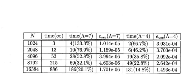
Table 2 shows the execution time and $e_{vec}$ for various numbers of vortex blobs. We

execute numerical computation with two

cases:

$\Lambda=7$ and $\Lambda=4$. $\delta$ is fixed to 0.01.

If

errors

of order $10^{-6}$ are tolerated, when _{$\Lambda=7,$$N=2^{14}$} yields

a

five times faster

computation.

3. desingularization parameter $(\delta)$:

Table3 shows evaluation

errors

withvarying$\delta$. Two

cases are

considered:(l) $N=4096$

and $\Lambda=8,$ (2) $N=16384$ and $\Lambda=8$

.

As $\delta$ increases, error gets smaller.

In order to make accurate computations, we need higher-order approximation. However,

since efficiency is reduced when $N$ is small, approximation order is restricted by the number

of vortex blobs. The

more

vortex blobs make accurate and effective computation possible.

From these results, we can conclude that this fast summation method is very effective when

$N$ and $\delta$ is large. These are already known in $[2, 3]$. However,

our

experiments seems to be

A time efficiency $e_{vec}$

$\ovalbox{\tt\small REJECT}_{1}^{4}1\infty 53000\%- 7470131361255110983228528\% 3994516\mathrm{e}066252149433761249351110_{70\% 25\mathrm{e}}928160453198\% 3038494\mathrm{e}-0^{6}7963215\% 3319052\mathrm{e}-0_{9}^{7}4\% 1265061\% 1135958\mathrm{e}- 02\% 2046922\mathrm{e}_{09}8\% 20928\% 2562842\mathrm{e}- 0\% 389558\mathrm{o}^{\mathrm{e}}\mathrm{e}-05\% 241796060607626- 044\mathrm{e}- \mathrm{e}- 0--050_{8}8$

Table 1: Execution time and evaluation

error

with various approximation order of Taylor

expansion A. $N=4096$ and $\delta=0.01$. $\infty$ means CPU time by direct summation. Efficiency

is lost, if $\Lambda\geq 12,$

.

$N$ time$(\infty)$ time$(\Lambda=7)$ $e_{vec}(\Lambda=7)$ time$(\Lambda=4)$ $e_{vec}(\Lambda=4)$

$\ovalbox{\tt\small REJECT}_{8}^{102}16384886186(201\%)1701\mathrm{e}-06131(40965328(528\%)3994\mathrm{e}- 06193582019424821513346109(32(1333\%)1014\mathrm{e}-052(667\%\%(769\%)1189\mathrm{e}- 056(46281\%)4603\mathrm{e}-0649(228\%)\% 370_{2}^{1}3\mathrm{e}- 04)2642\mathrm{e}-0(14\%)14\mathrm{e}044)30_{93-})209\mathrm{e}- 043\mathrm{e}- 04$

Table 2: Execution time and

error

when the number of vortex blobs $N$ is varied. $\Lambda=7$ and

4. $\delta=0.01$. $\mathrm{T}\mathrm{i}\mathrm{m}\mathrm{e}(\infty)$ is execution time using direct summation. Large number of vortex

$\delta$

$e_{vec}(N=4096)$ $e_{vec}(N=16384)$

$\ovalbox{\tt\small REJECT}_{2420_{9}}^{00}0104123106\mathrm{e}-01414214\mathrm{e}-- \mathrm{o}\mathrm{o}\mathrm{o}0004300_{6166}829185712078623\mathrm{e}-6065064376281271\mathrm{e}- 083\mathrm{e}-\mathrm{e}-\mathrm{e}- 06571300777392612488\mathrm{e}-0_{8}97626379870_{12\mathrm{e}}51298\mathrm{e}-07715\mathrm{e}07\mathrm{e}-\mathrm{o}- 08097$

Table 3: The relation between evaluation error $e_{ve\mathrm{c}}$ and desingularization parameter $\delta$. Two

combinations ofparameters; (1) $(\Lambda, N)=(8, 4096)$, and $(\Lambda, N)=(8, 16384)$

are

tested.

3.2

The

effect of changing variable

It is natural to ask if

we

need to change variables from $z$ to $w$. To show the effectiveness

of the change, we apply _{the fast summation algorithm to the discrete version to the original}

equation (1), too.

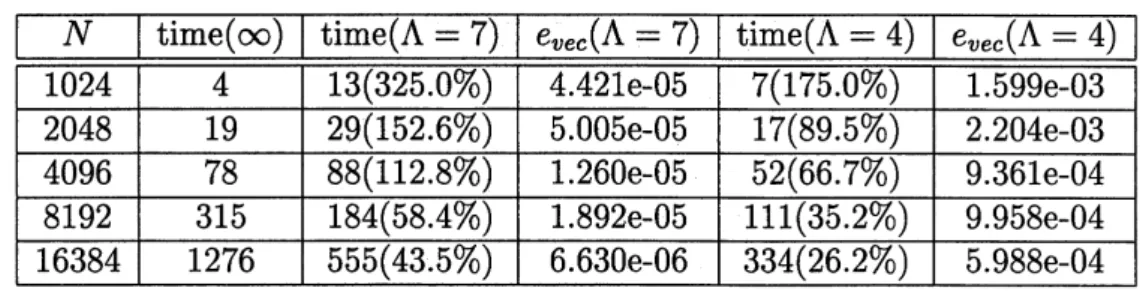
Table 4 is the list of execution time and

error

with various number of vortex blobs. $\Lambda=7$

and $\Lambda=4$

are

tested. $\delta$is fixed to 0.01. Timestep size for Runge-Kutta

method, $\triangle t$, is 0.01.

For small $N’ \mathrm{s}$, there is no advantage in using fast summation because of loss of efficiency.

If we compare Table 4 with Table 2, we

see

that the efficiency of Draghicescu’s algorithm

is improved very much by changing variables. One

reason

for this is as follows: Because of

periodic boundary condition, two points which are located at each edge of computational

domain ( ${\rm Re}[z]=0$ and ${\rm Re}[z]=1$ must be judged as those in near field. Some points which

were included in far field if it

were

not for the periodic boundary condition, are regarded as

those in near field. Consequently, number of points in nearfield increase, which is the reason

why it takes much time to evaluate the velocity field in original equation.

In addition to the

reason

above, there is another advantage of (2)

over

(1). In order

to approximate the vector field accurately

we

have to obtain higher order Taylor expansion

of the integral kernel. However, it is difficult to get higher order Taylor coefficients of the

integral kernel of (1), since it involves complicated combinations of trigonometric functions.

Even if we can obtain higher order Taylor coefficients, say, by

some

computer manipulation,

it

consumes

CPU time because ofverymany trigonometric function calls. Onthe otherhand,

we can easily obtain higher order coefficients of integral kernel of (2). Note that they are

rationalfunctions. Therefore, changing variable from $z$to$w$ makes it possibleto approximate

the kernel with little pain.

4

The

motion

of transformed

vortex

sheet

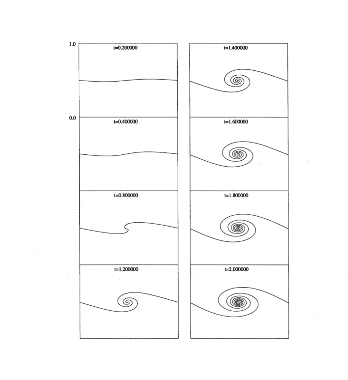
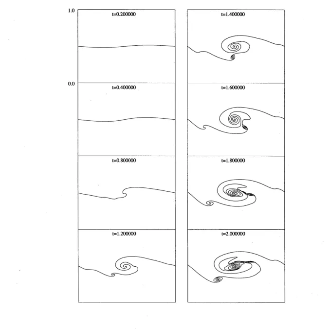
Figure 1 shows the time evolution of transformed vortex sheet by Draghicescu’s fast

$N$ time$(\infty)$ time$(\Lambda=7)$ $e_{vec}(\Lambda=7)$ time$(\Lambda=4)$ $e_{vec}(\Lambda=4)$

$\ovalbox{\tt\small REJECT}_{4}^{20}163841276555(35)6630\mathrm{e}-06334(262\%)5988\mathrm{e}- 40^{48}8110292967888(1128\% 4314131592184(584\% 9(32(15250_{\%}6\%)500_{2\mathrm{e}}^{1}5\mathrm{e}-\mathrm{o}_{5}\%)442\mathrm{e}-057(175)189-05111)126\mathrm{o}\mathrm{e}- 052517((667\%\%(352\%)9958\mathrm{e}-048950\%)15)9361\mathrm{e}- 04)2204\mathrm{e}- \mathrm{o}\mathrm{o}-499\mathrm{e}033$

Table 4: Execution time and evaluation

error

$e_{vec}$ with various $N$ when we apply

Draghicescu’s algorithm to the original equation of a vortex sheet with periodic boundary

condition. Desingularization parameter $\delta=0.01$. $\mathrm{T}\mathrm{i}\mathrm{m}\mathrm{e}(\infty)$ is execution time obtained by

direct summation.

and $\triangle t=0.05$

.

The equation (4) is solved with the initial condition (5). Fourier filter is not

used. While $t$ is small, the sheet is nearly flat. At about $t=0.8$ , vortex sheet begins to

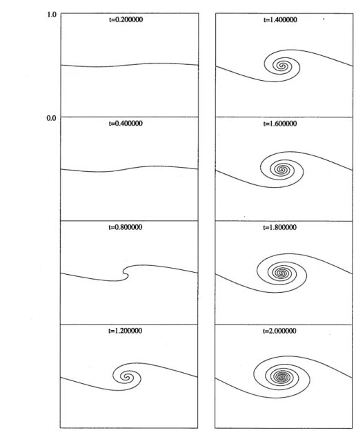
roll-up and a spiral grows afterwards. Figure 2 is the time evolution of transformed vortex

sheet by direct summation. When

we

compare these two figures,

no

difference is observed.

When we reduce A from 7 to 4, the numerical result is shown in Figure 3. In this case,

although its efficiency is

35.8%,

spurious spirals appear and complex pattern is formed by

vortex sheet at $t=2.0$

.

Thus $\Lambda=4$ is totally unacceptable

as a

numerical

mean.

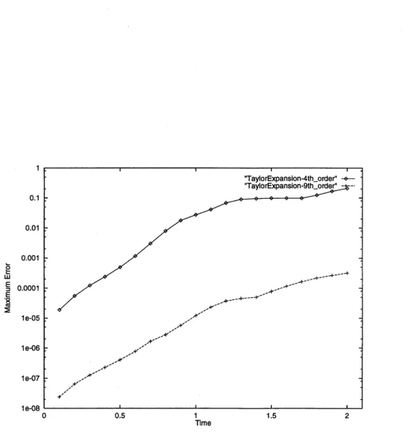
In order to study the accuracy, we define the position error, $e_{pos}$, as follows.

$e_{pos}=1\leq n\leq N\mathrm{m}\mathrm{a}\mathrm{x}|w_{n}^{fas}(tt)-w_{n}(direCt)t|$,

where $w_{n}^{fast}(t)$ and $w_{n}^{diect}(rt)$

are

the position of n-th vortex blob by Draghicescu’s fast

sum-mation and direct summation, respectively. In Figure 4, we show position

error

$e_{pos}$ when

$\Lambda=9$ and $\Lambda=4$

.

The position error is smaller than 0.0001 at $t=2.0$ when $\Lambda=9$

.

This

error seems

to be tolerable for

some

purposes.

We need more vortex blobs to compute accurately for a long time and to make efficiency

better. Figure 5 is the long time evolution when $(\Lambda, N)=(10, 8192)$. Other parameters

are

the same as before. In this case, we can compute up to $t=4.5$. A spiral gets bigger as time

grows. Efficiency is 46.0%.

5

Fourier

filter

As Krasny [7] notes, the numerical computations for small $\delta$ requires

a

technique called

Fourier filter. Figure 5 shows a reasonable computation, but we must note that this is

because, due to the largeness of $\Delta t(0.05)$, the number of iterations (90) is rather small,

hence the accumulation of evaluation

errors

is negligible. If$\triangle t$ issmall,

we

observe numerical

instabilityin early stages. AIso, if$\delta$ is small, numerical instability becomes obvious for small

Figure 1: The time evolution of transformed vortex sheet by Draghicescu’s fast evaluation.

Figure 2: The time evolution of transformed vortex sheet by direct summation. Numerical

Figure 3: The time evolution of transformed vortex sheet by Draghicescu’s fast method.

Numerical parameters: $N=4096,$ $\Lambda=4,$ $\delta=0.01$, and $\triangle t=0.05$. Because of the loss of

precision, the numerical solution is quite different from the directly evaluated solution for

Figure 4: The logarithm plotof evaluationerror$e_{pos}$ byfast algorithmwith$\Lambda=9$ and $\Lambda=4$.

Figure 5: The time evolution of transformed vortex sheet by Draghicescu’s fast method.

Numerical parameters: $N=8192,$ $\Lambda=10,$ $\delta=0.01$, and $\Delta t=0.05$. The increase of vortex

The present section is

Fourier filter works wellonly when the lowfrequencymodes

are

dominant and high frequency

modes decay sufficiently rapidly. In view ofthis,

we

consider the following initial condition:

$w_{n}(0)= \exp(\frac{2\pi\dot{i}n}{N})+\epsilon\exp(\frac{4\pi\dot{i}n}{N})$ $(n=1,2, \cdots, N)$,

where $\epsilon=0.01$

as

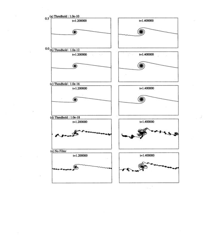
before.

We first study the effectiveness of the direct summation and the Fourier filter applied to

thetransformed equation (4). What wewant to cut off by the filter is round-offerror. Figure

6 shows the numerical solution of the sheet at $t=1.2$ and $t=1.4$, with thevarious threshold

value from $10^{-18}$ to $10^{-10}$ and without filtering. Numerical parameters are $N=8192,$ $\triangle t=$

O.Ol,and $\delta=0.01$. When Fourier filter is not applied, numerical solution is at $t=1.2$.

When the threshold is less than $10^{-18}$, round-off

error

can’t be cut off by the filter. As

a

result, round-off error is amplified and makes the numerical solution unstable. Therefore,

the threshold must be at least greater than $10^{-18}$. On the other hand, when the threshold is

equalto $10^{-10}$, numerical computation becomes unstable at$t=1.4$. This is because the filter

cutsoff the genuine increase of the modes. Consequently, to make accurate computation with

Fourier filter up to $t=1.4$, we find that it is desirable to choose the threshold value from

$10^{-16}$ to $10^{-12}$.

Next we apply Fourier filter to Draghicescu’s fast method. In this case, in addition to

round-off error, approximation

error

must be erased by the filter. However, approximation

error is much greater than round-off error. Therefore, unless the threshold value is chosen

properly, it isdifficult to cut off both

errors

by thefilter. Inorder tostudythe validthreshold,

we

give in Figure 7 logarithmic plots of Fourier coefficients of the numerical solution when

we proceed by one time step. Approximation order of each graph from top to bottom in the

Figure 7 is (a) A $=10,$ $(\mathrm{b})$ A $=12$, and (c) A _$=\infty$ (direct method), respectively. Other

parameters are $N=8192,$ $\triangle t=0.\mathrm{O}\mathrm{l},\mathrm{a}\mathrm{n}\mathrm{d}\delta=0.01$. This figure indicates that if we set the

threshold value to $10^{-12}$, the numerical errors of high frequency modes can’t be eliminated

in the

case

of$\Lambda=10$ and $\Lambda=12$.

Figure8is the time evolution of the sheet by Draghicescu’s fast method with Fourier filter.

Approximation order A is 12 and the threshold is $10^{-12}$. At $t=0.6$, numerical computation

doesn’t work well because of the failure of the filter. In order to cut off the errors surely the

threshold must be greater than $10^{-12}$, for example $10^{-10}$, which is found to be unsuitable in

the previous observation.

In order to usesmaller threshold, approximation error must be reduced. From the results

from section 3, there are three possibilities to improve accuracy of approximation;

$\bullet$ larger number of vortex blobs $(N)$ $\bullet$ higher order Taylor expansion $(\Lambda)$

In this paper, since the desingularized parameter $\delta$ is fixed to 0.01, we

use

larger $N$ and

higher order approximation, so that the effect of Fourier filter is compatible with efficiency.

Figure 9 shows the time evolution of the sheet. Numerical parameters

are

$N=$ _16384,

$\triangle t=0.01,$ $\delta=$ O.Ol,and A $=15$. The threshold value is $10^{-12}$. Efficiency is 42.3%. In

this combination of parameters, Draghicescu’s fast method with Fourier filter works well.

Therefore, Fourier filter is effective only when approximation error is sufficiently small, in

other words,

a

large number of vortex blobs

are

needed if

we

take efficiency into

considera-tion. From the viewpoint of practical application, this restriction is not serious because the

necessity of the fast method arises only when

we

want to

use.a

large number of vortex blobs.

Acknowledgment.

Theauthors began thepresentstudy bythe suggestion from $\mathrm{P}\mathrm{r}\mathrm{o}\mathrm{f}\mathrm{e}\mathrm{s}_{\vee}\mathrm{s}\mathrm{o}\mathrm{r}$R. $\mathrm{K}\mathrm{r}\mathrm{a}\mathrm{S}\mathrm{n}\mathrm{y}.$ We express

our

gratitude to Prof. R. Krasny, who kindly introduced to us Draghicescu’s algorithm as

References

[1] R.E. Caflisch and O. F. Orellana, Singular solutions and ill-posedness for the evolution

of vortex sheets, SIAM J. Math. Anal., vol. 20(1989), pp. 293-307.

[2] C.I. Draghicescu, An efficientimplementation of particle methodsfor the incompressible

Euler equations, SIAM J. Numer. Anal., vol. 31 (1994), pp. 1090-1108.

[3] C. I. Draghicescu and M. Draghicescu, A fast algorithm forvortex blob interactions, J.

Comput. Physics, vol. 116 (1995), p.

69-78.

[4] L. Greengard and V. Rokhlin, A fast algorithm for particle simulations, J. Comput.

Phys., vol. 73 (1987), pp. 325-348.

[5] J. Hamilton and G. Majda, On the Rokhlin-Greengard method with vortex blobs for

problems posed in all space

or

periodic in one direction, J. Comput. Phys., vol. 121

(1995), pp. 29-50.

[6] R. Krasny, A study of singularity formation in

a

vortex sheet by the point-vortex

ap-proximation, J. Fluid Mech., vol. 167 (1986), pp. 65-93.

[7] R. Krasny, Desingularization ofperiodic vortexsheet roll-up , J. Comput. Phys., vol. 65

(1986), pp. 292-313.

[8] R. Krasny, Computation of vortex sheet roll-up, Springer Lecture Notes in Math., $\#$

1360 (1988), Eds., C. Anderson and C. Greengard, pp. 9-22.

Figure 6: The numerical solution of transformed equation at t $=1.2$ and t $=1.4$ calcurated

by direct method with Fourier filter. Each

row

corresponds to the case of threshold value:

Figure 7: The logarithmic plot of Fourier coefficient of the numerical solution when we

proceed

one

time step. Numerical parameters; $N=8192,$ $\delta=0.01,\mathrm{a}\mathrm{n}\mathrm{d}\Delta t=0.\mathrm{O}1$.

Approxi-mation order in (a) and (b)

are

$\Lambda=10$ and $\Lambda=12$, respectively. In (c), we calcurated by

Figure 8: The time evolution of transformed vortex sheet using Draghicescu’s fast algorithm

with Fourier filter. Approximation order A is 12 and the threshold value is $10^{-12}$. Numerical

Figure 9: The time evolution of transformed vortex sheet using Draghicescu’s fast algorithm

with Fourier filter. $N=$ 16384. Approximation order A is 15 and the threshold value is