On Super Numerical Simulation (Discretization Methods and Numerical Algorithms for Differential Equations)

On Super Numerical

Simulation

Hitoshi IMAI (今井仁司), Toshiki TAKEUCHI (竹内敏己),

Hideo SAKAGUCHI (坂口秀雄) and Tetsuya HISHINUMA (菱沼哲也) \dagger

Faculty of Engineering, University of Tokushima, Tokushima 770-8506, Japan.

(徳島大学工学部)

\daggerGraduate School ofEngineering, University ofTokushima, Tokushima 770-8506, Japan.

(徳島大学大学院工学研究科)

1Introduction

Recently,

we can

easily

use

powerful computers. This year high-end PCs with $16\mathrm{G}\mathrm{B}$

mem-ory(chipset:E7500) or $64\mathrm{G}\mathrm{B}$ memory(chipset:GC-HE) are available. In next thirty years

computers will have more amillion times capability. What will be the future numerical

simulation ?Taking into consideration such development of computers,

we

propose apew

terminology: super numerical simulation. It means numerical simulation which highly

over-strides usual one. The similar terminology is seen in super computer. In what sense super numarical simulation should be super ?We propose five points: ultimate precision(

ul-timate reliability ), ulul-timate visualization, ultimate fast-computing, ultimate applicability,

and hardware implementation (cf. http:$//\mathrm{i}\mathrm{s}$am.$\mathrm{p}\mathrm{m}.\mathrm{t}\mathrm{o}\mathrm{k}\mathrm{u}\mathrm{s}\mathrm{h}\mathrm{i}\mathrm{m}\mathrm{a}-\mathrm{u}.\mathrm{a}\mathrm{c}.\mathrm{j}\mathrm{p}/\sim \mathrm{i}\mathrm{m}\mathrm{a}\mathrm{i}/$ ).

Hard-ware implementation

means

for example the flow simulator where the nural network

simu-latingflowis implemented ascircuitries. Amongthesefive pointsultimate precision, ultimate

visualization and ultimate applicability are shown in the paper.

2Ultimate

precision

In numerical simulation reliability of numerical solutions is checked by comparing those obtained in different precision. If numerical solutions converge, then it is recognized reliable

numerical solutions are obtained. However sometimes numerical solutions do not converge.

This is because they

are

not prepared abundantly. Usual numerical methods sometimes do not give abundant series of numerical solutions in different accuracy.

On the other hand, numerical simulation sometimes fails due to instability caused by

numerical

errors.

Especially, the rounding

error

plays afatal role. If the truncation

error

is

as

small

as

the rounding error, the rounding

error

spoils mathematical validity of the numerical method.

数理解析研究所講究録 1265 巻 2002 年 9-17

To

overcome

thesedifficulties

we

proposedIPNS(Infinite-Precision NumericalSimulation)

[6]. IPNS consists of the arbitrary order approximation method and the multiple precision arithmetic. The former is used for arbitrary reduction of the truncation

error.

The latter

is used for arbitrary reduction of the rounding error As the arbitrary order

approxima-tion method, spectral methods

are

available from the pratical view point[l]. Amongspectral

methodsSCM (SpectralCollocation Method) is very useful. Thisisbecausethewayofits

ap-plication issimilarasFDM. It iseasily applicable to nonlinear problemsincludingfree

bound-ary problems[ll]. Themultiple precision arithmetic is easily carried out by using free subrou-tine libraries on the net, e.g. http:$//\mathrm{w}\mathrm{w}\mathrm{w}$

.

$\mathrm{l}\mathrm{m}\mathrm{u}.\mathrm{e}\mathrm{d}\mathrm{u}/\mathrm{a}\mathrm{c}\mathrm{a}\mathrm{d}/\mathrm{p}\mathrm{e}\mathrm{r}\mathrm{s}\mathrm{o}\mathrm{n}\mathrm{a}\mathrm{l}/\mathrm{f}\mathrm{a}\mathrm{c}\mathrm{u}\mathrm{l}\mathrm{t}\mathrm{y}/\mathrm{d}\mathrm{m}\mathrm{s}\mathrm{m}\mathrm{i}\mathrm{t}\mathrm{h}2/$

FMLIB.html[10].

In the paper,

SCM

usingChebyshev Polynomials and Chebyshev-Gauss-Lobatto

colloca-tion points is used. Afunction $u(x)$ in [-1, 1] is approximated by the $N$-th order Chebyshev

Polynomials as follows:

$u(x)= \sum_{k=0}^{N}\tilde{u}_{k}T_{k}(x)$, _{$T_{k}(x)=\cos$}(k $\arccos x)$

.

(1)

There is

an

inversion formula

$u_{j}= \sum_{k=0}^{N}\tilde{u}_{k}T_{k}(x_{j})$, $\tilde{u}_{k}=\frac{2}{N\overline{c}_{k}}\sum_{j=0}^{N}\frac{1}{\overline{c}_{j}}u_{j}T_{k}(x_{j})$ (2)

where

$\overline{c}_{j}=\{$

2, $j=0$,$N$,

$x_{j}= \cos\frac{j\pi}{N}$, $j=0,1$,$\cdots$ ,$N$.

1otherwise, (3)

$\{x_{j}\}$ are called Chebyshev-Gauss-Lobatto collocation points. Derivatives at the collocation

points

are

easily computed from $\{u_{j}\}$

.

In SCM it is easy to increase the order of the

approx-imation by increasing the number of collocation points. This feature is quite remarkable and different from other discretization methods. Of

course

SCM is applicable both in space and

in time.

To see IPNS is realized, the following simple one-dimensional boundary value problem is

solved.

Problem 1. Find $u(x)$ s.t.

$u_{xx}=- \frac{\pi^{2}}{16}\sin\frac{(x+1)\pi}{4}$,

$-1<x<1$

, (4)

$u(-1)=0$, $u_{x}(1)=0$. (5)

Remark 1. The exact solution to Problem 1is $u(x)= \sin\frac{(x+1)\pi}{4}$

.

Numerical results are shown in Table 1. Here $(N+1)$ Chebyshev-Gauss-Lobatto points

are

used. Extremely high accuracy is obseved. It should be remarked that even to such asimple

problem IPNS needs huge memory spaces and too much computational time

now.

Table 1. Maximum

error

for Problem 1.(2500 digit numbers)

3Ultimate visualization

In numerical simulation visualization is very important. However, in super numerical

simu-lation normal visualization may not be available. For example IPNS gives numerical datain

long digits. There is no visualization softwarewhich can deal with such data. Among highly

accurate results by IPNS difference is extremely small. There is no visualization software

which can show such small difference.

Here anew visualization for IPNS is presented. Multiple precision arithmetic is used in

pre-processing which is programed in FORTRAN. Then suitable data whose regulation is

given by the visualization software are created and delivered to the visualization software.

Some examples obtained by the new visualization

are

shown below. It is interesting that

basic facts in numerical analysis

are

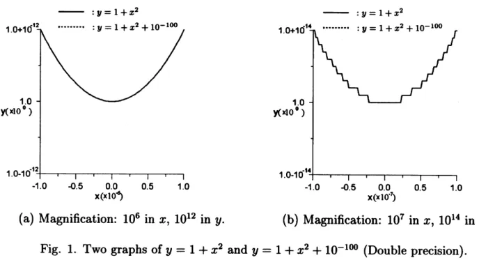
visualized.

Fig. 1shows two graphs of $y=1+x^{2}$ _and $y=1+x^{2}+10^{-100}$ in different

magnifica-tion. Graphs are generated by connecting $(x_{j}, y(x_{j}))_{j=0}^{100}$ in astraight line, $\{x_{j}\}$

are

equally

distributed. Data are prepared in double precision. Two graphs are not distinguished. This is because $10^{-100}$ is neglected compared with $1+x^{2}$

.

Fig. 1(b) shows machine epsilon

or

distribution of floating-point numbers

–: y$=1+x^{2}$ _–:y$=1+x^{2}$

(a) Magnification: 10 in x, 10 in y. (b) Magnification: 10 in x, 10 in y.

Fig. 1. Two graphs of y $=1+x^{2}$ and y $=1+x^{2}+10^{-100}$ _{(Double precision).}

Fig. 2shows two graphs of $y=1+x^{2}$ _and $y=1+x^{2}+10^{-100}$ _{in different} magnifica-tion. Graphs

are

generated by connecting $(x_{j},\tilde{y}(x_{j}))_{j=0}^{100}$ in astraight line, $\{x_{j}\}$

are

equally

distributed. $\tilde{y}(x)$ is theinterpolated function by SCM with _{$(x:, y(x:))_{i=0}^{10}$}, _$\{x:\}$ :

Chebyshev-Gauss-Lobatto Collocation points in [-1, 1]. Data

are

prepared in double precision. Two graphs

are

not distinguished. This is because 10 is neglected compared with $1+x^{2}$

.

In

Fig. $2(\mathrm{b})$ oscillation to be induced from the rounding

error

is

seen.

– :y$=1+x^{2}$ – :y$=1+x^{2}$

(a) Magnification: 10 in x, 10 in y. (b) Magnification: 10 in x, 10 in y.

Fig. 2. Two graphs ofinterpolated functions created by SCM with data from y $=1+x^{2}$

and y $=1+x^{2}+10^{-100}$ _{(Double precision).}

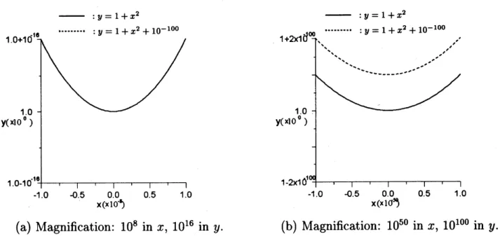
Fig. 3shows the new visualization for two graphs of $y=1+x^{2}$ _and $y=1^{\backslash }+x^{2}+$ $10^{-100}$ in (jifferent magnification. Graphs

are

generated by connecting $(x_{j},\tilde{y}(x_{j}))_{j=0}^{100}$ in a

straight line, $\{x_{j}\}$ are equally distributed. $\tilde{y}(x)$ is the interpolated function by SCM with

$(x_{i}, y(x_{i}))_{i=0}^{10}$, $\{x_{i}\}$ : Chebyshev-Gauss-Lobatto Collocation points in [-1, 1]. Data

are

prepared in 200 digit numbers. In Fig. $3(\mathrm{b})$ two graphs are very natural and distinguished

from each other.

– :$y=1+x^{2}$ – :_$y=1+x^{2}$

(a) Magnification: 10 in $x$, 10 in $y$. (b) Magnification: 10 in $x$, 10 in $y$

.

Fig. 3. Two graphs ofinterpolated functions created by SCM with data from $y=1+x^{2}$ and $y=1+x^{2}+10^{-100}$ (200 digits).

4Ultimate applicability

Inverse problems often arise from practical problems. It is well-known they are very difficult to besolved[3]. Their directsimulation has been ataboo due to easycorruption bythestrong

oscillation phenomenon. To avoid this oscillation phenomenon

some

additional methods

are

usually used together. To say roughly, these are regularization[12], the method of least

squares and $\mathrm{A}\mathrm{I}$

.

Restriction of the dimension of the solution space is asort of regularization.

These methods

are

very useful but unfortunately not absolute. Especially, in numerical simulation the rounding

error

fails their theoretical usefulness.

On the other hand, direct simulation by IPNS was applied to several inverse problems governed by PDE systems[4, 5, 7, 8]. Numerical results were very satisfactory. This

means

numerical

errors

are extremely small,

so

they do not induce the oscillation phenomenon. In

the paper the following integral equation of the first kind with

an

analytic kernel and an

analytic solution is solved by IPNS without any additional methods like regularization$[2, 5]$.

Problem 2. Find $u(y)$ s.t.

$\int_{-1}^{1}e^{xy}u(y)dy=f(x)$, $f(x)= \frac{(2x-1)e^{x}+e^{-x}}{2x^{2}}$, _$f(0)=1$

.

(6)

Remark 2. The exact solution to Problem 2is $u(y)= \frac{y+1}{2}$.

SCM is applied to the integrand

as

follows:

$e^{xy}u(y) \cong\sum_{k=0}^{N}\tilde{g}_{k}(x)T_{k}(y)$

.

(7)

From the inversion formula

$\tilde{g}_{k}(x)\cong\frac{2}{Nc_{k}}\sum_{j=0}^{N}\frac{1}{c_{j}}e^{xy_{\mathrm{j}}}u_{j}T_{k}(y_{j})$, k $=0,$ 1,

\cdots , N, (8)

where

$y_{j}= \cos\frac{j\pi}{N}$, _{$u_{j}=u(y_{j})$}, j _$=0,$ 1,

\cdots , N. (9) Thus $e^{xy}u(y) \cong\sum_{k=0}^{N}\frac{2}{Nc_{k}}\sum_{j=0}^{N}\frac{1}{c_{j}}e^{xy_{\mathrm{j}}}u_{j}T_{k}(y_{j})T_{k}(y)$

.

(10) Then $\int_{-1}^{1}e^{xy}u(y)dy\cong\int_{-1}^{1}\{\sum_{k=0}^{N}\frac{2}{Nc_{k}}\sum_{j=0}^{N}\frac{1}{c_{j}}e^{xy_{\mathrm{j}}}u_{j}T_{k}(y_{j})T_{k}(y)\}dy$ $= \frac{2}{N}\sum_{k=0}^{N}\sum_{j=0}^{N}\frac{1}{c_{k}c_{j}}e^{xy_{\mathrm{j}}}u_{j}T_{k}(y_{j})\int_{-1}^{1}T_{k}(y)dy$ (11) $= \frac{2}{N}\sum_{k\neq 1}^{N}\sum_{jk=0=0}^{N}\frac{1}{c_{k}c_{j}}e^{xy_{\mathrm{j}}}u_{j}\cos\frac{jk\pi}{N}\cdot\frac{1+(-1)^{k}}{1-k^{2}}$

.

We choose properly points $\{x_{l}\}$, $l=0,1$, $\cdots$ , $N$

on

which the integral equation is

satisfied. Set $f_{l}=f(x_{l})$, then

we

have the following linear system:

$\sum_{j=0}^{N}a_{lj}u_{j}=\frac{N}{2}f_{l}$, $\mathit{1}=0,1$,$\cdots$ , $N$, (12)

14

$a_{lj}= \sum_{k=0,k\neq 1’}^{N}\frac{1}{c_{k}c_{j}}e^{x_{l}y_{\mathrm{j}}}\cos\frac{jk\pi}{N}\cdot\frac{1+(-1)^{k}}{1-k^{2}}$. (13)

After solving this linear system, $u(y)$ is reconstructed

as

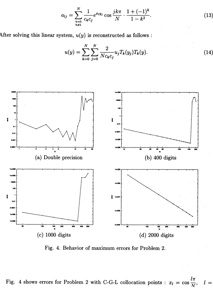
follows :

$u(y)= \sum_{k=0}^{N}\sum_{j=0}^{N}\frac{2}{Nc_{k}c_{j}}u_{j}T_{k}(y_{j})T_{k}(y)$. (14)

$\xi$

$\not\in$

(a) Double precision (b) 400 digits

$\not\in$

1

(c) 1000 digits (d) 2000 digits

Fig. 4. Behavior of maximum

errors

for Problem 2.

Fig. 4shows

errors

for Problem 2with C-G-L collocation points : $x_{l}= \cos\frac{l\pi}{\mathrm{w}}$, _$l=$

15

0, 1, \cdots ,N. Here,

error

$= \max_{0\leqq j\leqq N}|u_{N}(y_{j})-u(y_{j})|$, $y_{j}= \cos\frac{j\pi}{N}$, $\dot{\gamma}=0,$1,\cdots ,N (15)

$u(y)$ is the exact solution, and $u_{N}(y)$ is the right-hand side ofEq. (14). If rounding

error

is

notsmall enough,

error

growsexplosivelybeforeobtaining good results. This shows the linear

system (12) is very ill-conditioned. Atthe

same

time, ifrounding

error

is smallenough,

error

reduces successively

as

$N$ becomes large. In Fig. $4(\mathrm{d})$ the regression line by the method of

least squaresis $\log$(error) $=-3.00*\log N$ 0.686 with the correlationcoefficient _$\rho=-3.00$

.

This

means

IPNS works well.

5Conclusion

In the paperanew terminology: super numericalsimulation isproposed. Severalexamples of super numerical simulation

are

also presented. As computers become

more

powerful today’s super numerical simulation becomes normal. However, super numerical simulation exists at

any time, as super computer exists at any time.

Acknowledgements

This work ispartially supported byGrants-in-Aids for Scientific Research (No. 13640119), from the Japan Society of Promotion ofScience.

References

[1] C. Canutoet al., Spectral Methods in Fluid Dynamics, Springer, 1998.

[2] H. Fujiwara and Y. Iso, NumericalChallengeto fll-posedProblems byFastMultiple PrecisionSystem,

Proc. the 50th Japan National Congress on Theoretical and Applied Mechanics, 2001, 419-424.

[3] G. Hammerlin et al., ImproperlyPosed Problems and Their Numerical Treatment, Birkh\"auser, 1983.

[4] H. Imai and T. Takeuchi, Application of the Infinite Precision Numerical Simulation to an Inverse

Problem, NIFS-PROC-40(1999), 38-47.

[5] H. Imaiand T. Takeuchi, Some AdvancedApplications of the SpectralCollocationMethod, GAKUTO

Int. Ser. Math. Sci. Appl., 17(2001), 323-335.

[6] H. Imai, T. Takeuchi and M. Kushida, On Numerical Simulation of Partial Differential Equations in

Infinite Precision, Advances in Mathematical Sciencesand Applications, $9(2)(1999)$, _1007-1016.

[7] H. Imai, T. Takeuchi, M. Nakamura and N. Ishimura, ADIRECT APPROACH TO AN INVERSE

PROBLEM, GAKUTOInt. Ser. Math. Sci. Appl., 12(1999), 223232.

[8] H. Imai, T. Takeuchi and H. Sakaguchi, Infinite Precision Numerical Simulation for PDE Systems and

Its Applications, RIMSKokyuroku, Kyoto University, 1147(2000),42-50

[9] D. E. Knuth, The Art of Computer Programming, Addison-Wesley, 1981.

[10] D. M. Smith, AFORTRAN Package For Floating-Point Multiple-Precision Arithmetic, Tran

on Mathematical Software, 17(1991), 273-283.

[11] Tarmizi, T.Takeuchi, H. Imai andM. Kushida, Numerical simulation of one-dimensional free$\mathrm{b}_{1}$

problems ininfinite precision, Advancesin MathematicalSciencesand Applications, 10(2)

672.

[12] A. N. Tikhonov and V. Y. Arsenin, Solution of$\Pi 1$-Posed Problems, John Wiley&Sons, 1977