A Simple Near Optimal Parallel Algorithm for Recognizing Outerplanar Graphs

A

Simple Near Optimal Parallel Algorithm for Recognizing

Outerplanar Graphs

Shin-ichi

Nakayama (中山慎–) Shigeru Masuyama (増山繁)

Department of

Knowledge-Based

Information Engineering, Toyohashi University of Technology

Toyohashi-shi, Aichi 441, Japan

E–mail: [email protected], [email protected]

Abstract. Anouterplanargraph isa graph whichcanbeembedded inthe planesothat allverticeslieonthe boundary of theexteriorface. Inthis paper, wepropose asimple

near optimal parallel algorithm forrecognizingwhether a givengraph$G$isouterplanar

in $O(\log n)$ time using $O(n\alpha(l, n)/\log n)$ processors on an arbitrary-CRCW PRAM

where $n$ is the number of vertices in $G,$ $\alpha(l, n)$ is the inverse Ackermann function,

which growsextremely slowly with respect to $l$ and _$n[9]$ and $l=O(n)$. Although a

near optimal parallel algorithmfor general graphs can also beobtained bycombining the algorithm in [3] with the algorithm for finding biconnected $\mathrm{c}\mathrm{o}\mathrm{m}_{\mathrm{P}}\mathrm{o}\mathrm{n}\mathrm{e}\mathrm{n}\mathrm{t}\mathrm{s}[4][9]$ , our

algorithmuses methods completely different from the algorithm in $[3]’ \mathrm{s}$ and is much

simpler than $[3])\mathrm{s}$.

1

Introduction

An outerplanar graph is an undirected graph which can be embedded in the plane in such a way that all vertices lie on the exterior face(, see Fig. 1). A graph always denotes an undirected graph throughout this paper, except when it is specified to be directed. For outerplanar graphs, several efficient algorithms for solving

important problems e.g., vertex-coloring, edge-coloring, longest path, are known $[9][5]$

.

Fur-thermore, it is well-known that a given graph is outerplanar if and only if a given graph has

pagenumberone, wheregraph$G$haspage

num-ber one if there exists a linear arrangement of verticesso that no pair of edges is crossing when they are drawn on the same side of the lin-ear arrangement of the vertices $[13][11]$

.

The

problem of deciding whether a given graph has

pagenumberone is the special case of the book embedding, whose application to fault-tolerant VLSI design is described e.g., in the introduc-tion of [13]. Thus, it is useful to develop effi-cient algorithms for recognizing whether a given graph is outerplanar or not.

Mitchell [10] proposed an $O(n)$ sequential

algorithm for recognizing outerplanar graphs where $n$ is the number of vertices in $G$

.

The

sequential algorithm removes a vertex $v$

sat-isfying some properties from a given graph $G$

step by step, and cannot straightforwardly be

applied to develop an efficient parallel algo-rithm. Diks, Hagerup and Rytter [3] devel-oped a parallel algorithm for recognizing

out-erplanar graphs. When an input graph is bi-connected, the algorithm [3] runs in $O(\log n)$

time using $O(n/\log n)$ processors on a CRCW

PRAM (, see e.g., [8]), where $n$ is the

num-ber of vertices in $G$

.

However, when an input

graph is a general graph, we need to find bi-connectedcomponentsbefore applying the algo-rithm [3] to each biconnected component. The best known parallel algorithm for finding bicon-nected components runs in $O(\log n)$ time

us-ing $O((n+m)\alpha(m, n)/\log n)$ processors on the

arbitrary-CRCW PRAM [4] [9] where $m$ is the number of edges and $\alpha(m, n)$ is theinverse

Ack-ermannfunction, which growsextremely slowly

with respect to $m$ and $n[9]$

.

\dagger The

arbitrary-CRCW PRAM is defined by the property that when several processorstry towrite tothesame memory cell in the same step, then exactly one of them succeeds [8]. As outerplanar graphs haveat most $2n-3$edges [10], by checking this fact first, we can find biconnected components

in $O(\log n)$time using$O(n\alpha(l, n)/\log n)$

proces-sors on the arbitrary-CRCW PRAM where $l=$ $O(n)$

.

Thus, the algorithm _[3] combined with

the algorithm for finding biconnected

compo-nents [4] [9] takes, in total, $O(\log n)$ time using $O(n\alpha(l, n)/\log n)$ processors on the

arbitrary-CRCWPRAM, when appliedtogeneral graphs. Similarly, on a CREW PRAM(, see e.g., [8]),

the complexityofparallel algorithm [3] is

domi-natedby

_fin.

ding $\mathrm{b}\mathrm{i}_{\mathrm{C}\mathrm{O}}\mathrm{n}.\mathrm{n}$ectedcomponents,when

applied to general graphs.

In this paper, we present a simple near

optimal parallel algorithm for recognizing

outerplanar graphs in $O(\log n)$ time using

\dagger If_{the class of input graphs is linearly contractible} graph class [7] such as the class of planargraphs, an

optimal parallelalgorithm for finding biconnected

com-ponentsthatruns in$O(\log n)$time using$O(n/\log n)$ pro-cessors on the arbitrary-CRCW PRAM exists [7].

How-ever, this algorithm does not work for general graphs.

$O(n\alpha(l, n)/\log n)$ processors on the

arbitrary-CRCW PRAM, in the sense that $O(\log n)\cross$ $O(n\alpha(l, n)/\log n)=O(n\alpha(l, n))$ is almost

lin-ear with respect to $n$

.

Although anear optimal

parallelalgorithm for general graphs can also be obtained bycombining the algorithm in [3] with the algorithm in [4] [9],our algorithm uses meth-ods completely different from the algorithm in

$[3]’ \mathrm{s}$, e.g., the well known _$st$-numbering, and is

much simpler than $[3]’ \mathrm{s}$

.

2

Definitions

Given an undirected connected graph $G=$

(V,$E$) having no multiple edges. A path $P$

from $v_{0}$ to $v_{k}$ in $G$ is a finite non-null

se-quence $v_{0},$$e_{1},$$v_{1},$$e2,$ $v2,$$\cdots,$$e_{k},$ $v_{k},$ $v_{i}\in V,$ $i=$

$0,1,$ $\cdots,$$k,$ $e_{j}\in E,$ $j=1,2,$$\cdots,$$k$, such that,

for $1\leq i\leq k$, the end vertices of $e_{i}$ are $v_{i-1}$

and $v_{i}$, respectively. If _{$v_{0}=v_{k}$}, then path $P$ is

a circuit.

A biconnected graph $G$ is a connected graph

whichhasnovertex$v$suchthat$G-v$ (thegraph

obtained byremoving$v$from $G$) hasatleasttwo

connected components. A biconnected

outer-planar graph hasa planar embedding consisting of a circuit bounding the exterior face, where

(possibly) a number of non-crossing edges are embedded within the interior region of this cir-cuit [5]. Edges on the boundary of the exterior face are called sides, while the other edges are called diagonals [5].

Next, we describe the $st$-numbering used in our parallel algorithm.

Definition 1 [12] An $st$-numbering is a one-to-onefunction $f$from$V$to$\{1, \cdots, n\}$ satisfying the following twoconditions :

(ii) for each $v\in V-\{s,t\}$, there exist

adja-centvertices$v_{1}$ and$v_{2}$such that$f(v_{1})<f(v)<$

$f(v_{2})$

.

Fig. 2 illustrates $st$-numbering. The st-numbering is used as an indispensable

compo-nent in several algorithms [12]. We have the following theorem.

Theorem 1 [$\mathit{1}\mathit{2}f$ A graph $G$ is biconnected

if

and only

_if

it has an $st$-numbering by letting

$s=u$ and $t=v$

for

each edge $(u, v)$

.

(Note 2.1) If graph $G$ is biconnected, its

st-numbering can be obtained in $O(\log n)$ time

using $O((n+m)\alpha(m, n)/\log n)$ processors [4]

where $n$ (resp., $m$) is the number of vertices

(resp., edges) in $G$ and $\alpha(m, n)$ is the inverse Ackermann function.

3

The

Parallel

Algorithm

We first assumethat the given graph $G$is

bicon-nected. We shall describe how to treat general graphs at the end of this section. The following theorems characterize outerplanar graphs. Theorem 2 $f\theta$] Given graph $G=(V, E),$ $G$

is outerplanar

_if

and only

_if

$G$ has no subgmph

homeomorphic to either $K_{4}$ or $K_{2,3}$, where $K_{4}$

is the complete graph on

_four

vertices and $K_{2,3}$

is the graph illustrated in Fig. 3. $\square$

Theorem 3 $f\mathit{1}\mathit{0}f$ An outerplanar graph $G$

with $n(\geq 3)$ vertices has (i) at most $2n-3$ edges,

(ii) at least two vertices

_of

degree 2. $\square$

Our parallel algorithm first checks, based on Theorem 3, if $G$ has at most $2n-3$ edges and

at least two vertices of degree 2. Then, this al-gorithm chooses a vertex $v$ of degree 2 and a

vertex $v’$ incident to $v$; regards $v$ (resp., $v’$) as $s$ (resp., $t$) and finds $st$-numbering of $G$

.

Note

that, by Note 2.1 just after Theorem 1, we can find $st$-numbering of $G$ because $G$ is assumed

to be biconnected. When $G$ is outerplanar,

ex-actly one Hamiltonian circuit always exists in

$G$, and the edges constructing the Hamiltonian

circuit can be regarded as sides of the

outerpla-nar graph $[2][5]$

.

Consequently, the above $\mathrm{p}\mathrm{r}\mathrm{c}\succ$

cess finds the sides by the following lemma. In the following, suppose that the vertices in$G$ are

numbered from 1 to $n$ by$st$-numbering where$s$

is avertexofdegree 2 and $t$ is a vertex incident

to $s$ and each vertex in $G$ is identified with its

vertexnumber.

Lemma 1

_If

$G$ is outerplanar; then alledges

$(i, i+1),$ $i=1,$$\cdots,$$n-1$, are in $G$

.

(proof) We shall show that, if$G$ does not have

some edge among $(\dot{i}, i+1),$ $i=1,$$\cdots,$$n-1$,

then $G$ is not outerplanar. Assume that

ver-tex $i$ is not incident to vertex $\mathrm{i}+1$

.

By the

definition of $st$-numbering, each vertex $x,$ $x=$

$2,$$\cdots,$$n-1$, must be incidentto avertexwhose

number is less than $x$ and to a vertex whose

number is more than $x$, respectively. By this

fact and the connectivity of $G,$ $G$ has simple

path $P_{i,s}$ $=i,j_{1},j_{2},$$\cdots,j\iota,$$s$, $(l\geq 1)$ where

$i>j_{1}>j_{2}>\cdots>j_{l}>1(=s)$

.

Vertex 1

$(=s)$ is adjacent to exactly two vertices $n(=t)$

and 2 by definition, so $j_{l}$ of $P_{i,s}$ must be 2$($,

see Fig. 4). Similarly, for $\mathrm{i}+1$, simple path

$P_{i+1,s}$ $=i+1,j_{1}’,j_{2}’,$$\cdot\cdot,$$,j’\iota$

” $s,$ $(l’\geq 1)$ where

$i+1>j_{1}’>j_{2}’>\cdots>2(=j_{\iota’},)>1(=s)$exists.

Moreover, bythefact that eachvertex$x,$ $x=$

whose number is more than $x,$ $G$ has simple

paths$P_{i,t}=i,$$k_{1},$ $k_{2},$$\cdots,t$, where$i<k_{1}<k_{2}<$

$<t(=n)$, and $P_{i+1,t}=i+1,$$k_{1’ 2}’k’,$_$\cdots,$$t$,

where $i+1<k_{1}’<k_{2}’<\cdots<t(=n)$

.

Since $t>\cdots>k_{2}>k_{1}>i>j_{1}>j_{2}>$ $>j_{l}>1(=s),$ $P_{i,t}$ and $P_{i,s}$ share no vertex

except $i$

.

Similarly, _{$P_{i,t}$} and

$P_{i+1,s},$ $P_{i+1,t}$ and

$P_{i,s},$ $P_{i+1,t}$ and $P_{i+1,s}$ share no vertex except $i$,

$\dot{i}+1$

.

$G^{*}$, constructed by _{$P_{i},,$${}_{s}P_{i+1},S’ Pi,t$} and

$P_{i+1,t}$, has a subgraph homeomorphic to $K_{2,3}$

(, see Fig 4). Hence, $G$ is not outerplanar by

Theorem 2, which however contradicts the

as-sumption that $G$ is outerplanar. Thus we have

shown that if $G$ is outerplanar, then $G$ has all

edges $(i,\dot{i}+1),$ $i=1,$$\cdots$,$n-1$

.

$\square$

By Lemma 1, if at least one edge among

$(i, i+1),$ $i=1,$$\cdots,$$n-1$, does not exist in $G$, then the algorithm stops since $G$is not

out-erplanar, otherwise the edges $(i, i+1),$ $i=$

$1,$_$\cdots,$$n-1$, and _{$(n, 1)$} construct a Hamiltonian

circuit $C$

.

We regard the edges constructing $C$

as sides of the outerplanar graph. (Note that if $G$ is outerplanar, Hamiltonian circuit _$C$ is

unique [5]. )

We assume that $C$ is embedded in the plane

so that each edge of$C$ bound the exterior face and the edges of

$G-C(G-C$

denotes the graph obtained by removing edges of $C$ from $G)$ are embedded within the interior region of $C$

.

The edges of$G-C$ are called _$di,a$gonals of

$G$

.

If the diagonals do not intersect each other

onsuch embedded edges, then$G$is outerplanar,

otherwise $G$ is not outerplanar.

Tosee this, weexecute the following process. Hereafter, we identify each vertex with its

ver-tex number assigned by st-numbering.

Let$M(i),$$i=1,$ $\cdots,$ $n$, be an array such that

$M(i)$ contains _vertex$j_{0}$ where $j_{0} \equiv\min\{j|j$

is the endpoint of diagonals adjacent to $i$

}.

If there is no diagonal incident to $i,$ $M(i)$ has

a value $+\infty$ where $+\infty$ is a sufficiently large

number $\mathrm{s}\mathrm{a}\mathrm{t}\mathrm{i}\mathrm{s}\mathrm{f}\mathrm{y}\mathrm{i}\mathrm{n}\mathrm{g}+\infty>n$

.

For each diagonal

$(x, y)$ such that _$x<y$, we execute $val(x, y)arrow$ $\min\{M(i)|x\leq i\leq y\}$ _{and regard} $val(x, y)$

as the value of diagonal $(x,y)$

.

On the value

$val(x, y)$ for each diagonal $(x, y)$, we obtain the

following lemma.

Lemma 2 Assume that Hamiltonian circuit $C$ is embedded in the plane so that each edge

of

$C$ bounds the exterior

face

and diagonals are embedded within the interiorregion

_of

$C$

.

The diagonals intersect each other

_if

andonly

if

there is a diagonal $(x, y)$, where_$x<y$, such

that the value $val(x, y)$ is less than vertex num-$berx$

.

(proof) $(\Rightarrow)$ Assume that there is a pair of

diagonals which intersect each other. Let $(x, y)$, $(x’, y’)$, where _{$x<y,$ $x’<y’$} and $x’<x$, be

a pair of intersecting diagonals. As these two diagonals intersect each other, vertex $y’\mathrm{s}\mathrm{a}\mathrm{t}\mathrm{i}_{\mathrm{S}}-$

fies

$x<y’<y$

and is adjacent to diagonal

$(x’, y)’$ where $x’<x$ (See Fig. $6(\mathrm{a})$). Hence,

$val(x, y)= \min\{M(i)|x\leq i\leq y\}<x$

.

$(\Leftarrow)$ Assume thatno diagonals intersect each

other. Since no diagonals intersect each other,

each vertex $j$ adjacent to vertex $\dot{i}$, where

$x\leq$

$i\leq y$, satisfies $x\leq j\leq y$ for each diagonal $(x, y)$ where $x<y$ (See Fig. $6(\mathrm{b})$). Hence,

$val(x, y)= \min\{M(i)|x\leq i\leq y\}\geq x$

.

$\square$

In the following, we introduce Procedure Recognition for recognizing whether a given graph is outerplanar.

Proced$\mathrm{u}$re Recognition

begin

The list ranking algorithm [8] can handle

steps1,2 in$O(\log n)$timeusing$O(n/\log n)$

pro-(Step 1) if $m>2n-3$,

then print “_{$G$is not outerplanar” and}

stop.

(Step 2) if $G$does not haveatleasttwovertices

ofdegree 2,

then print “_{$G$is not outerplanar” and}

stop.

(Step 3) Choose a vertex $v$ of degree 2 and a

vertex $v’$ incident to $v$; regard $v$ and $v’$ as $s$ and $t$, respectively, and find an

$st$-numbering of$G[12][4]$

.

(Step4) if$G$ does not have at least one edge

among $(i, i+1)$ for all $i,$ $1\leq i\leq$

$n-1$, where $i,$$i+1$ are the vertex

numbers assigned by Step 3,

then print “_{$G$is not outerplanar” and}

stop.

(Step 5) For each vertex $i,$ $i=1,$ $\cdots,$ $n$,

$M( \dot{i})\vdash\min\{j|j$ is the endpoint of

diagonals adjacent to $i$

}.

(Step 6) For each diagonal $e_{j}=(x, y)$ where

$x<y$,

$val(x, y) arrow\min\{M(i)|x\leq i\leq y\}$

(Step 7) if there is a diagonal $(x, y)$, where

$x<y$, such that $val(x, y)<x$, then print “_{$G$ is not outerplanar”,} else print “_{$G$ is outerplanar”.}

end. $\square$

The correctness of Procedure Recognition is obvious by Theorem 3 and Lemmas 1 and 2. We then analyze the computation time and the number of processors required.

The$\mathrm{c}.0$mplexity analysis is done under the

as-sumption that each vertex of theinput graph$G$

has a pointer to its predefined adjacency list,

that is, for each vertex $v\in V$, the vertices

ad-jacent to vertex $v$ are given in a liked list, say, $L[v]=\langle u_{1}, u_{2}, \cdots, u_{d}\rangle$, in some order, where $d$is the degree of$v$ (Fig. $5(\mathrm{a})$). Recall that the

arbitrary-CRCW PRAM is used as a parallel computation model in this paper.

cessors.

Notethat $m=O(n)$ in the following analysis,

assteps 3-7 are executed only when $m\leq 2n-3$

by step 1.

Theparallel algorithm for finding st-numbering runs in$O(\log n)$time using$O((n+m)\alpha(m, n)/\log n)$

processors [4] where $n$ (resp., $m$) is the

num-ber of vertices (resp., edges) in input graphs and $\alpha(m, n)$ is the inverse Ackermann func-tion. Thus, in step 3, finding $st$-numbering of$G$

requires $O(\log n)$ time using $O(n\alpha(l, n)/\log n)$

processors where $l=O(n)$

.

After finding the $st$-numbering, each of the

initial vertex numbers in the adjacency lists

$L[\iota]’ \mathrm{s}$ is replaced by its number assigned by the

$st$-numbering. For this process, we first

trans-form the adjacency lists $L[i]’ \mathrm{s}$ into a linked list

$L’$asfollows. Let a vertex$u_{d}^{i}$ bethe last element

in the adjacency list$L[i]$ of vertex$i$and avertex

$u_{1}^{i+1}$ the first element in $L[i+1]$

.

Each vertex

$u_{d}^{i}$ has a pointer to $u_{1}^{i+1}$, for $i=1,$

$\cdots,$ $n-1$,

(See Fig. $5(\mathrm{b})$). We then convert the linked list

$L’$ into an array $A$ by applying the list

rank-ing algorithm [8] which runs in $O(\log n)$ time

using $O(n/\log n)$ processors. And we replace

each of the initial vertex numbers by its

num-ber assigned by$st$-numbering using a standard

technique used to implement Brent’s schedul-ing $\mathrm{p}\mathrm{r}\mathrm{i}\mathrm{n}\mathrm{C}\mathrm{i}_{\mathrm{P}}1\mathrm{e}[5][8]$ as follows. Partition elements

of $A$ into equal-sized blocks $E_{i},$ $i=1$, ,

$|A|/\log n$, where each size is $O(\log n)$

.

Treat

each block $E_{i}$ separately, and sequentially

re-place each of the initialvertex numbers belong-ing to block $E_{i}$ by its number assigned by

st-numbering. This process runs in $O(\log n)$ time

Step 4runsin$O(\log n)$ timeusing$O(n/\log n)$

processors by applying Brent’s scheduling

$\mathrm{p}\mathrm{r}\mathrm{i}\mathrm{n}\mathrm{c}\mathrm{i}\mathrm{p}\mathrm{l}\mathrm{e}[5][8]$ stated in step 3.

Let $A[k, k’],$ _{$1\leq k<k’\leq|A|(=O(n))$ be}

an interval between $k$ and $k’$ in $A$

.

Note that

the elements in $A$ are numbers assigned by

st-numbering. As the degree of each vertex is found in step 2, we can recognize the vertices

adjacent to vertex $v$ as the element in

inter-val $A[k, k’]$ where $1\leq k<k’\leq|A|$

.

For

ex-ample, assume that $d_{i}$ is the degree of vertex $i$, the vertices adjacent to vertex 1 are the

ele-ments in $A[1, d_{1}]$, the vertices adjacent to ver-tex2 are the elements in $A[d_{1}+1, d_{1}+d_{2}]$, and

so on. (Note: Given the degree of each

ver-tex, the intervals in $A$ corresponding to vertex

$i$ for $i=1,$

$\cdots,$ $n$, are found in $O(\log n)$ time

using $O(n/\log n)$ processors by applying

prefix-sums algorithm [8]. ) Hence, in step 5, finding each minimum vertex number adjacent to ver-tex$i$ for $i=1,$

$\cdots,$ $n$, can be done by

comput-ing the minimum of interval in $A$ corresponding

to vertex $i$

.

As described in [8]

$(\mathrm{p}\mathrm{p}$

.

131-136$)$,

after executing a preprocessing algorithm

(AL-GORITHM 3.8 in [8]$)$ which runs in $O(\log n)$

time using $O(n/\log n)$ processors, we can

com-pute the minimum $A_{\min}[k_{i}, k_{i}’]$ of$A[k_{i}, k_{i}’]$, that

is, $\min\{A(k_{i}), A(k_{i}+1), \cdots, A(k_{i}’)\}$, where

1 $\leq$ $k_{i}$ $<$ $k_{i}’$ $\leq$ $|A|$, in $O(1)$ time using

$O(1)$ processors. We need to compute the

minimum $A_{\min}[k_{i}, k’]_{\mathrm{S}}i$’ corresponding to vertex $i,$ $i=1,$ _$\cdots,$ $n$

.

Hence, by Brent’s

schedul-ing $\mathrm{p}\mathrm{r}\mathrm{i}\mathrm{n}\mathrm{c}\mathrm{i}\mathrm{p}\mathrm{l}\mathrm{e}[5][8]$, we can compute the

mini-mum$A_{\min}[k_{i}, k’]_{\mathrm{S}}i$’ for $i=1,$ _$\cdots,$ $n$, in $O(\log n)$

time using $O(n/\log n)$ processors. The total

complexity in step 5 is $O(\log n)$ time using

$O(n/\log n)$ processors.

In step 6, we compute $\min\{M(i)|x\leq$

$i\leq y$ $\}$, where

$x<y$

, for each diagonal

$e_{j}=(x, y),$ $j=1,$ $\cdots,$ $k(=O(n))$

.

Since this

process is equivalent to the process described in step 5, this can be done in $O(\log n)$ time using

$O(n/\log n)$ processors.

Step 7 takes $O(\log n)$ time using $O(n/\log n)$

processors.

Having assumed that the input graph $G$ is a

biconnected graph sofar, we shalldescribe,

be-fore closing this section, how to decide whether

$G$ is outerplanar when $G$ is a general graph.

We first check if $G$ has at most $2n-3$ edges.

We next find biconnected components, that

is, blocks $B_{1},$ $B_{2},$$\cdots,$$B_{k}$ of $G$ by applying the

algorithm of finding biconnected components

in [4] [9], which runs in $O(\log n)$ time using $O(n\alpha(l, n)/\log n)$ processors. If $G$ is

outerpla-nar, then each of blocks $B_{1},$$B_{2},$ $\cdots$ ,$B_{k}$ is also

outerplanar [2]. Thus, we independently exe-cute Procedure Recognition for each of these blocks $B_{1},$ $B_{2},$_$\cdots,$$B_{k}$

.

If a block$B_{i}$ is an edge,

then ProcedureRecognition tells that $B_{i}$ is

out-erplanar. When each block $B_{i},$ $i=1,$_$\cdots,$$k$,

is outerplanar, we print “_{$G$is outerplanar” and}

stop. By the above-mentioned statements, we

have thefollowing theorem.

Theorem 4 Given a graph $G$ with $n$

ver-tices and $m$ edges, whether $G$ is outerplanar

or not can be decided in $O(\log n)$ time using $O(n\alpha(l, n)/\log n)$ processors on the

arbitrary-CRCW PRAMwhere$\alpha(l, n)$ is the inverse

Ack-ermannfunction, which grows extremely slowly

with respect to $l$ and

References

[1] R. Cole, U. Vishkin: “Approximate

par-allel scheduling, II:

_Ap.

plications to opti-mal parallel graph algorithms in logarith-mic time”,

_Inform.

Comput., 91, PP.1-47,

1991.

[2] K. Diks: “A fast parallel algorithm for six-coloring ofplanar graphs”, LNCS 233,

Springer Verlag, pp.273-282, 1985.

[3] K. Diks, T. Hagerup, and W. Rytter: “Op-timal parallel algorithms for the recog-nition and coloring outerplanar graphs”,

LNCS 379, Springer Verlag, pp.207-217,

1989.

[4] D. Fussell, V. Ramachandran and R.

Thurimalla: “Finding triconnected

com-[10] S. L.Mitchell: “Linear algorithmsto recog-nize outerplanar and maximal outerplanar graphs”,

_Information

Processing Letters, 9,

pp.229-232, 1979.

[11] S. Masuyama,S. Naito: “Decidingwhether graph G has page number one is in

NC”,

_Information

Processing Letters, 32,

pp.199-204, 1992.

[12] Y. Maon, B. Schieber and U. Vishkin: “Parallel ear decomposition search (EDS) and $\mathrm{s}\mathrm{t}$-numbering in graphs”, Theoretical

ComputerScience, 47, pp.277-298, 1986.

[13] M. Yannakakis: “Embedding planar graphs in four pages”, J. Comput. System Sci., 38, pp.36-67, 1989.

ponents by local replacement”, SIAM J. Comput., 22, 3 , pp.587-616, 1993.

[5] A. Gibbons and W. Rytter:

_Efficient

Par-allel Algorithms, Cambridge University

Press, 1988.

[6] F. Harary: Graph Theory,

Addison-Wesley, 1969.

[7] T. Hagerup: “Optimal parallel algorithms of planar graphs”,

_Inform.

Comput., 84,

pp.71-96, 1990.

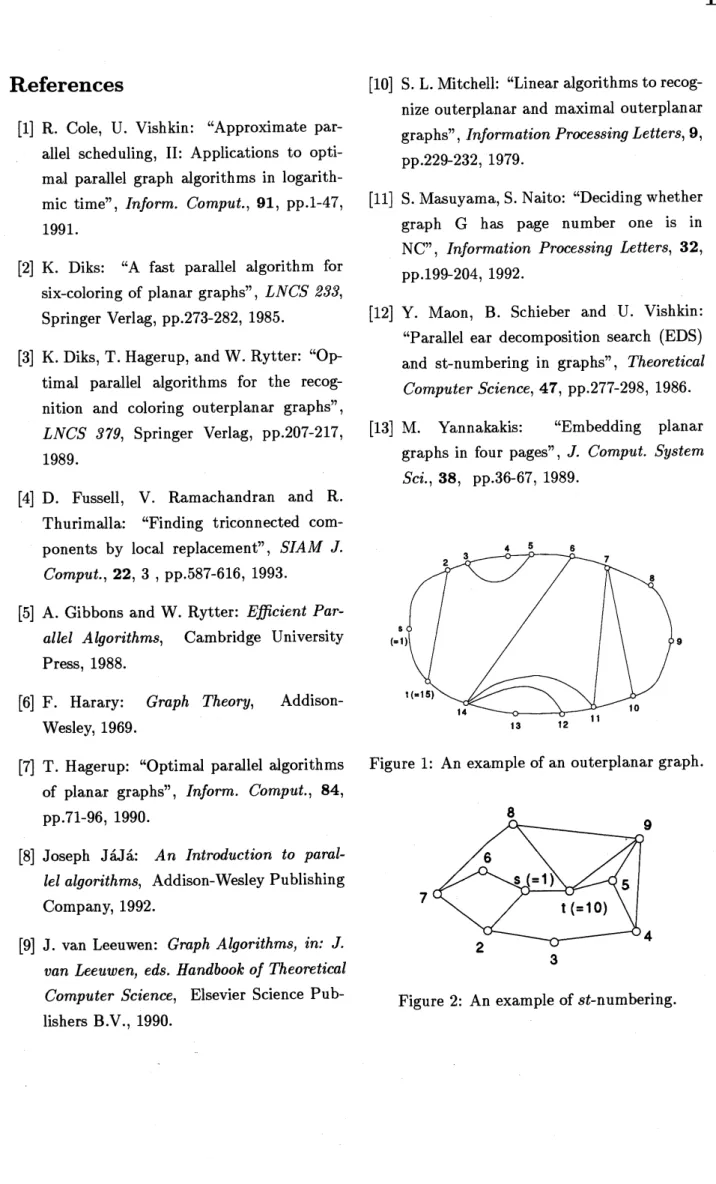
Figure 1: An example of an outerplanar graph.

[8] Joseph J\’aJ\’a: An Introduction to paral-lel algorithms, Addison-Wesley Publishing Company, 1992.

[9] J. van Leeuwen: Graph Algorithms, in: J. van Leeuwen, eds. Handbook

_of

Theoretical

Computer Science, Elsevier Science Pub-lishers B.V., 1990.

.q-. $K_{00_{-}}$

(a)L (b)L

5: Adiarpnrv liqt.$.\mathrm{q}T,/i$) i

$=1,$ \cdots , n, and linked list $L’$

.

{0’