Sulfur Chemical State and Chemical Composition of Insoluble Substance in Soft Rime, Hard Rime, and Snow Collected in Remote and Rural Areas in Japan Using Wavelength-dispersive X-ray Fluorescence

全文

(1)ANALYTICAL SCIENCES MAY 2018, VOL. 34. 589. 2018 © The Japan Society for Analytical Chemistry. Sulfur Chemical State and Chemical Composition of Insoluble Substance in Soft Rime, Hard Rime, and Snow Collected in Remote and Rural Areas in Japan Using Wavelength-dispersive X-ray Fluorescence Shoji IMAI,*1† Yuhei YAMAMOTO,*1 Takashi YAMAMOTO,*1 Kenji KODAMA,*2 Jun NISHIMOTO,*3 and Yoichi KIKUCHI*4 *1 Division of Chemistry, Institute of Natural Science, Graduate School of Technology, Industrial and Social Sciences, Tokushima University, 2-1 Minamijosanjima-cho, Tokushima 770–8506, Japan *2 X-ray Instrument Division, Rigaku Corporation, 14-8 Akaoji-cho, Takatsuki, Osaka 569–1146, Japan *3 Department of Environmental Sciences, Faculty of Life and Environmental Sciences, Prefectural University of Hiroshima, 562 Nanatsuka, Shobara, Hiroshima 727–0023, Japan *4 Laboratory of Chemistry, Faculty of Education, Iwate University, 3-18-33 Ueda, Morioka, Iwate 020–8550, Japan. Using a commercially available wavelength-dispersive X-ray fluorescence (WDXRF) spectrometer, the chemical composition and S-Kα spectrum of rime and snow samples collected in remote and rural areas of Japan were measured with a membrane filter sample technique to investigate the long-range transport of aerosol from the East Asian continent. Insoluble substances are derived into three categories: 1) conventional mineral origin (crustal substance), 2) urban dust origin (Fe-Zn-Ca) and 3) coal origin (S-As). Assuming that (i) S(VI) was found as a plaster-like substance in hard rime, depending on [Ca], and that (ii) S(-II) was found as non-crustal sulfur compounds, fractions of S(VI) and S(-II) in rime could be calculated as 35 ± 6 and 66 ± 7% by [Ca], which is in agreement with 32 ± 8 and 68 ± 8%, respectively, by the chemical shift of the S-Kα line. During a one-day meteorological event that included the accumulation of both rime and snow, differences to the snow-like content corresponded to characteristics typical of rime since the chemical compositions of rime also includes the composition of the snow. The fractions of 22 ± 12% of S(VI) and 76 ± 12% of S(-II), respectively, were found in rime. The fraction of S(-II) decreased from the Chugoku district towards the Shikoku district. Along the coast of the Japan Sea, the fraction of S(-II) decreased from Chugoku district toward the Northeast Japan. It can be proposed that other analytical techniques of S, Al, and Ca in that are favorable to this fractionation. Keywords Speciation, sulfur, WDXRF, chemical shift, rime, snow, aerosol, wet deposition, remote area (Received June 9, 2017; Accepted January 9, 2018; Published May 10, 2018). Introduction There is a long history of studying the long-range transport of air pollutants over the Japan Sea from Northeast Asia, from the viewpoint of their significant risk to human health and the environment.1–3 Zhao et al. reported on the risks from coal combustion exhaust in 1988.4 Rapid increases in the population and economic development increased the emission of atmospheric pollutants. In cities in the North of China, central heating systems with coal as their main energy source are widely used for residences in winter and are operated by local governments with no effective exhaust emission control systems. The winter monsoon plays an important role in long-range transport from the northeastern area of China (including Shandong, Shanxi, Hebei, Liaoning, Jilin, and Heilongjiang). An interesting report was published by Yang et al.5 The To whom correspondence should be addressed. E-mail: [email protected]. †. composition of polycyclic aromatic hydrocarbons (PAHs) in airborne particulate matter collected at Wajima, on the Noto Peninsula, Ishikawa, Japan was similar to that in Shenyang in the winter, but not in Kanazawa, strongly suggesting that PAHs produced by coal combustion in Northeast China were transported over the Japan Sea. The PAHs are categorized as incompletely burned carbonaceous substances. Another proof of the long-range transport of Chinese coal combustion exhaust is based on studies of the isotope ratios of 34S6,7 and Pb.8 Recently, airborne particulate matter, such as PM2.5, transported from China, became a focus of attention in Japan. Coal combustion with no exhaust purification specifically emits: 1) aerosol particulates including As, Cd, Pb and Zn; 2) gaseous pollutants, such as SO2, 3) products of incomplete combustion, and 4) inorganic small spherical particles (ISPs) from power plants. Zhong and Chun9 reported that in the urban area of Beijing and the industrial areas of Shenyang, the distributed aerosol particle sizes were 0.5 – 1.8, 2 – 8 and 10 – 15 μm; however, in rural areas, the sizes were approximately 15 μm. During the winter, particles of 0.5 – 1.0 μm included.

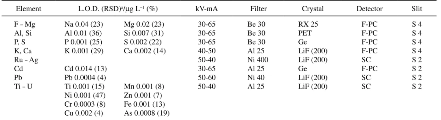
(2) 590 higher concentrations of air pollutants, such as S, Zn, Pb, and As.9 Gaseous SO2 is converted to non-sea-salt sulfate (nss-SO4) during long-range transport over the Japan Sea.10 Itabashi et al.10 reported on a seasonal variation of sulfur pollutants in the eastern Asian region. In Shikoku Island, Japan, the conversion rate of gaseous SO2 generated in China is about 80% or more during the winter, and the contribution from China is 60 – 70% of the total nss-SO4. Nagafuchi et al. reported a black acidic rime ice collected on the remote island of Yakushima, Japan, a World Heritage Area, transported from Shandong and Shanxi, China. In the black filtrate, inorganic ash spheres (glassy spheres, IAS) and spheroidal carbonaceous particles (SCP) were found by SEM-EDS observation. The IAS were mainly composed of Si and Al, while the SCP consisted of elemental carbon. Tanabe et al.11 reported that sulfur in the aerosol particles from Shenyang, China included the S(IV) form and that those from Harbin or Shenyang were mainly in the S(VI) form. Ban et al. reported an S(-II) species in coal fly ash and urban dust in Beijing.12,13 Calkins14 reported that organic sulfur compounds, such as thiophene and its derivatives, are also primarily included in the coal and are produced by its pyrolysis, because of their thermally stability up to 950° C, while thiophene, benzothiophene and dibenzothiophene are decomposed with 25, 19, and 10% efficiencies, respectively. Shi et al.15 reported that the levels of carbonaceous materials and mineral particles were comparable in aerosols from urban areas, suburban areas and the clean air district in Beijing, but that coal fly ash was higher in the clean air district. Recently, Imai et al.16–19 classified the ISPs included in insoluble rime, hard rime, and snow into five categories, with their chemical components corresponding to their area of generation: AREA-A, Huabei-type; AREA-B, Dongbei-type; AREA-B2, Korean peninsula-type; AREA-C, Heilongjiang-Russia-type, and AREA-D, Japan-type. When the winter monsoon is predominant, the S(-II) compounds were transported from northeast China together with various components of coal combustion exhaust from similar areas of ISP generation. Airborne particulate matter having sizes of 0.1 – 0.5 μm (accumulation mode) effectively forms condensation nuclei for ice crystal formation (ice nuclei). Particulates become attached to ice crystals growing in snow clouds. This scavenging phenomenon is known as in-cloud scavenging (snowout). Below the snow cloud, particulates in the atmosphere adhere directly as snow falls as so-called below-cloud scavenging (washout). Hard rime with a smooth surface is formed by direct deposition of overcooled water aerosols in the wind direction on any objects at temperatures under –10° C near the 1500 m altitude of the bottom of the snow cloud. Airborne particulate matter enters the hard rime ice as condensation nuclei. In the case of rime (soft rime), this could be considered to be an advantage with respect to the deposition of particulates due to the “shrimp-tail” morphology of the textured surface of rime. Its textured surface is advantageous for direct inertial collision of airborne particulate and dust during exposure to cold air flow from winter monsoon in the transition layer. Larger particulates are deposited more efficiently and effectively. Although XAFS techniques are powerful tools for analyzing the chemical state of sulfur,20 achieving good results typically requires a synchrotron radiation source, which makes it difficult to perform routine analytical work using this technique at present. Determining the chemical state of sulfur in coal from S-Kβ spectra obtained by wavelength dispersive X-ray fluorescence spectroscopy (WDXRF) has a long history as a useful method.21–23 Gohshi et al.24 reported the effectiveness of S-Kα spectra for analyzing coke and its associated corrosion. ANALYTICAL SCIENCES MAY 2018, VOL. 34 product. Many workers25–28 also reported that the chemical shift of the S-Kα line is effective on determining the chemical form of sulfur. Due to its economically efficient performance and short operating times, WDXRF as a technique for determining chemical speciation has become significant in the research field of cross-border air pollution events. The aim of this work is to use WDXRF to provide a methodology for the sulfur speciation of airborne particles, including the origin and/or fractions of S(VI) and S(-II), determined from the combination of (i) the ratio of the elemental components of the filtrates and (ii) the chemical shift of the S-Kα line.17–20 The application of this methodology is interesting in terms of its applicability to other elements.. Experimental Reagents and chemicals Commercially available sodium sulfate (Na2SO4), sodium hydrogen sulfate (NaHSO4), sodium sulfite (Na2SO3), sodium hydrogen sulfite (NaHSO3), sodium thiosulfate (Na2S2O3), and cysteine reagents were purchased from Nacalai Tesque Co., Ltd., Kyoto and were used as standards for the WDXRF analysis (chemical shift of the S-Kα line). Coal fly ash was obtained from two independent power plants in Japan. A certified reference material, AIST GSJ JCFA-1 coal fly ash, was also used. Instruments A Rigaku ZSX PrimusII WDXRF spectrometer (Rigaku Corp., Tokyo, Japan), equipped with SQX analytical software based on a fundamental parameter (FP) method, was used for samples deposited on a membrane filter. The standard operating conditions, the limit of detection (LOD), and its RSD% are summarized in Table 1. Figure S1 (Supporting Information) shows a typical WDXRF spectrum of an insoluble rime. The analytical result with the FP method was confirmed with the standard reference material, NIST 2783. The recoveries of Si, Al, K and Ti, so-called common crustal elements, were 106.2, 88.8, 92.1, and 102.3%, respectively. Those of Fe, Ca, S, Zn, and Pb, so-called non-crustal elements, were 97.7, 95.1, 91.1, 107.4, and 98.0%, respectively. These elements were selected in this work. Conventional multiple measurement by WDXRF was difficult due to damage to the sample, as this changed its properties. A Hitachi SEM-TM3000 (Hitachi High-Technologies) equipped with a Swift ED3000 EDX system was used at 15.0 kV with a collection time of 30.0 s. An ADVANTEC membrane mixed cellulose ester filter No. A045A047A (d 47 mm, pore size 0.45 μm) was used to filter rime and snow samples. Location Figure 1 shows the locations of sampling sites Nos. 1 – 12: No. 1, Mt. Kajigamori, Kochi Prefecture (1399 m); No. 2, Mt. Tsurugizan, Tokushima Prefecture (1955 m); No. 3, Mt. Osorakan, Hiroshima Prefecture (1330 and 850 m); No. 4, Nanatsuka, Shobara City, Hiroshima Prefecture (315 m); No. 5, Hiruzen Kogen, Okayama Prefecture (530 m); No. 6, Mt. Hachibuse, Hyogo Prefecture (1200 m); No. 7, Mt. Taikoyama, Tango Peninsula, Kyoto (650 m); No. 8, Yokokura, Katsuyama City, Fukui Prefecture (410 m); No. 9, Mt. Dainichigatake, Gifu Prefecture (1260 m); No. 10, Mt. Hishigatake, Yasuzuka, Jouetsu City, Niigata Prefecture (960 m); No. 11, Mt. Iwateyama, Shizukuishi, Iwate Prefecture (1200 m); No. 12, Mt. Shimokura, Hachimantai City, Iwate Prefecture (1130 m). Table S1 (Supporting.

(3) ANALYTICAL SCIENCES MAY 2018, VOL. 34. 591. Table 1 Instrumental conditions for the FP method Element F – Mg Al, Si P, S K, Ca Ru – Ag Cd Pb Ti – U. L.O.D. (RSD)a/μg L–1 (%) Na 0.04 (23) Al 0.01 (36) P 0.001 (25) K 0.001 (29). Mg 0.02 (23) Si 0.007 (31) S 0.002 (22) Ca 0.002 (14). Cd 0.014 (13) Pb 0.0004 (4) Ti 0.001 (15) Ni 0.001 (47) Cr 0.0003 (8) Cu 0.002 (4). Mn 0.001 (8) Zn 0.001 (7) Fe 0.001 (13) As 0.0008 (19). kV-mA. Filter. Crystal. Detector. Slit. 30-65 30-65 30-65 40-50 50-40 30-65 50-60 50-40. Be 30 Be 30 Be 30 Al 25 Ni 400 Al 25 Ni 40 Al 25. RX 25 PET Ge LiF (200) LiF (200) Ge LiF (200) LiF (200). F-PC F-PC F-PC F-PC SC F-PC SC SC. S4 S4 S4 S4 S2 S2 S2 S2. Target, Rh; X-ray path, vacuum; measurement time (Cr, Cu, As, Se, Cd, Hg, Pb), peak = 4 s, BG = 4 s. a. Relative standard deviation of limit of detection based on S/N ratio.. Results and Discussion. Fig. 1 Locations of sampling site. No. for sampling: 1, Mt. Kajigamori; 2, Mt. Tsurugizan; 3, Mt. Osorakan; 4, Shobara Nanatsuka; 5, Hiruzen Kogen; 6, Mt. Hachibuseyama; 7, Tango Peninsula; 8, Yokokura, Katsuyam; 9, Mt. Dainitigatake; 10, Mt. Hishiagatake; 11, Mt. Iwatesan; 12, Mt. Shimokurayama.. Information) shows the latitude and longitude of sampling sites.16 Rime samples can be only collected from Nos. 1 and 2. Sampling Fresh snow samples were collected using a polyethylene vat at 1 m above the ground levels covered by snow at sampling site No. 1. At this site, fresh snow can collect near the bottom of snow clouds, and the influence of below-cloud scavenging may be neglected at its 1400 m altitude. However, rime also accumulated on sampling nets that were exposed to cold air masses. The soft and hard rime accumulating on the SUS304 net was collected carefully without physically damaging the net. The Fe, Cr, and Ni contents were measured as below the LODs for the rime samples; this is supported by SEM observations from our previous reports.18,19 To suppress the effect of meteorological factors, both rime and snow were allowed to accumulate in the late-night/early hours of a day and were collected early in the morning. At No. 2, the soft rime accumulating on a nylon rope was collected without damaging the rope. At high altitude sites of Nos. 3, 6, 9, 10, 11, and 12 and Nos. 4, 7, and 8 in clean rural areas, fresh snow was collected from the basal snow layer.. SEM observation of insoluble substrates of snow and rime Figures 2(a) and 2(b) show SEM images of insoluble substrates of snow (498 g) and rime (106 g), respectively. Both snow and the accumulated rime were collected at No. 1 in the early hours of Jan. 22, 2014. Minerals and IPSs were observed in both images. The amounts of whole size and larger size particles in the rime sample were more than in the snow sample. Figure 2(d) shows an SEM image and a photo image of the rime membrane collected after four days exposure to cold air flow at No. 1, whose rime was formed on Feb. 19, 2013, as shown in the SEM image and photo image in Fig. 2(c). Both filtrates were obtained from 500 g of sample. Drastic increases in the amounts of mineral and IPS particles were clearly observed, and the filter became black, reflecting exposure to the cold air mass. This represents significant evidence of the below-cloud scavenging effect (direct inertial collision) of the aerosol particles in the atmosphere below the cloud altitude. Therefore, this can be considered as an advantage with respect to the deposition of particulate matter based on the “shrimp-tail” morphology of rime. The SEM-EDX observation shown in Fig. S2 (Supporting Information) indicates a large sulfur content in the ISPs. Although Ban et al. reported the presence of sulfur species S(-II) in coal fly ash and urban dust in Beijing,12,13 it was impossible to deduce the presence of S(-II) species from the EDX. Chemical composition of the insoluble substance Table 2 gives the average content and standard deviation (ave. ± sd) in units of μmol L–1, an enrichment factor for the crustal component, a factor of the content normalized to [Al], and the ratio of rime/snow normalized for the elements Si, Al, K, Ca, S, Ti, Zn, As, and Pb. The contents of element M in rime and snow are defined as [M]rime and [M]snow, and its contents rime snow and [M]Al , normalized to [Al] are defined as [M]Al respectively. The enrichment factor, EF, normalized by the crust components S, As, and Pb, exceeded the average of 0.52 ± 0.33 for the common crustal origins to be Si, Al, K and Ti, where crust components were based on reported chemical components in the interior of the North China Craton.29 An enrichment in rime was observed for the elements originating from coal, S, As, and Pb. In the case of Fe and Zn, which depended on urban dust, slight enrichment was observed only in rime. The ratios of rime snow /[M]Al for the common crustal elements were within the [M]Al average value of 1.12 ± 0.13. The ratios of As and Pb did not.

(4) 592. ANALYTICAL SCIENCES MAY 2018, VOL. 34. Fig. 2 SEM-image of insoluble species on filter and photograph of the membrane filter. (a) Rime 500 g at Feb. 19, 2013 (×5000, ×3000); (b) rime 500 g at Feb. 23, 2013 (×5000, ×3000); (c) snow 498 g; (d) rime 106 g at Jan. 22, 2014 (×6000).. Table 2 Chemical composition of insoluble substances Snow (n = 25) Element. Rime (n = 6). Average ± S.D./ Average ± S.D./ E.F. E.F. mol L–1 mol L–1. Crustal Si 83.6 ± 99.2 Al 36.1 ± 43.3 K 2.21 ± 3.22 Ti 0.283 ± 0.392 Non-crustal Fe 2.19 ± 2.77 Ca 0.524 ± 0.736 S 0.351 ± 0.386 Zn 0.013 ± 0.028 As 0.0028 ± 0.0045 Pb 0.0034 ± 0.0049. 0.56 1.00 0.27 0.26. 391.9 ± 198.2 173.5 ± 76.2 13.2 ± 10 1.54 ± 0.87. 0.38 18.3 ± 8.46 0.02 3.58 ± 1.61 1.21 2.91 ± 1.37 0.90 0.082 ± 0.074 2.41 0.0150 ± 0.0094 2.67 0.0157 ± 0.0082. Ratio rims [M]Al snow [M]Al. 0.54 1.00 0.34 0.30. 0.98 1.00 1.24 1.13. 0.65 0.03 2.08 1.18 2.69 2.91. 1.74 1.42 1.73 1.31 1.11 1.09. sample crust /[M]Al . E.F.: Enrichment factor = [M]Al. increase beyond this average. Similar crustal species of As and Pb are deposited in rime and snow. Fe, Ca, and S exceeded the average, indicating a concentrating effect of non-crustal substances in rime. The plot of a binary system and the resulting correlations provide important information about the origins of the insoluble substances. Plots of [M] vs. [Al] of the snow and rime samples together with the coal fly ash produced by the coal fired power plants in Japan are shown in Fig. S3 (Supporting Information). The determination coefficients (r2), which are the squares of the correlation coefficients (r), were divided into three categories: Category 1) r2 > 0.9 for Si, K, Fe, Ca, and Ti; Category 2). 0.8 > r2 > 0.5 for S and As; Category 3) r2 < 0.2 for Zn. Where for Fe, Ca, S, Zn, and As, [Si]snow = 2.110 × [Al]snow – 1.791. r2 = 0.9940 (1). [Fe]snow = 5.207 × 10–2 × [Al]snow – 0.1431. r2 = 0.9736 (2). [Ca]snow = 1.575 × 10–2 × [Al]snow – 0.09437 r2 = 0.9118 (3) [S]snow = 6.778 × 10–3 × [Al]snow + 0.07470. r2 = 0.6539 (4). [Zn]snow = 9.31 × 10–5 × [Al]snow + 0.00515. r2 = 0.0998 (5). [As]snow = 4.79 × 10–5 × [Al]snow + 0.000177 r2 = 0.7900 (6) [Pb]snow = 6.54 × 10–5 × [Al]snow + 0.000556 r2 = 0.8356 (7) The plots of the [M] vs. [Si] of snow were, [Al]snow = 3.991 × 10–1 × [Si]snow + 4.115. r2 = 0.8663 (8). [Fe]snow = 2.463 × 10–2 × [Si]snow – 0.09830. r2 = 0.9764 (9). [Ca]snow = 7.425 × 10–3 × [Si]snow – 0.07795 r2 = 0.8995 (10) [S]snow = 3.212 × 10–3 × [Si]snow + 0.08047. r2 = 0.6580 (11). [Zn]snow = 1.03 × 10–4 × [Si]snow + 0.00479 r2 = 0.1380 (12) [As]snow = 2.29 × 10–5 × [Si]snow + 0.000199 r2 = 0.5947 (13) [Pb]snow = 3.10 × 10–5 × [Si]snow – 0.000505 r2 = 0.8425 (14).

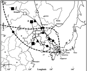
(5) ANALYTICAL SCIENCES MAY 2018, VOL. 34 Table 3 Correlation coefficient (r) components of the rime at No. 1 site. Fe Ca S Zn As Pb. between. 593. non-crustal. Fe. Ca. S. Zn. As. Pb. *. 0.879 *. 0.514 0.728 *. 0.865 0.946 0.876 *. 0.707 0.548 0.922 0.963 *. 0.490 0.100 0.469 0.003 0.173 *. The points for rime (Fe, S, Zn, and As) were plotted above their regression line, but those of coal fly ash were on or near the regression line. In all cases, for the hard rime samples at No. 1 and rime at No. 2, the data were distributed on the regression line. The results for rime are systematically above the regression line, indicating the presence of a characteristic substance in it. The content of snow origin of M in rime ([s.o.-M]rime), was estimated from the mean values of snow origin, [s.o.-MAl]rime and [s.o.-MSi]rime, which were calculated from [Al]rime and [Si]rime using Eqs. (1) to (14). [s.o.-M]rime = 0.5([s.o.-MAl]rime + [s.o.-MSi]rime). (15). The excess [M] is defined as [ex.M]rime = [M]rime – [s.o.-M]rime,. Fig. 3 Back trajectory of aire mass from 1500 m alt. on No. 1. a, Dec. 24, 2014; b, Jan. 22, 2014; c, Feb. 16, 2014; d, Feb. 21, 2014; e, Dec. 28, 2014; f, Nov. 28, 2013 on No. 2. ○, 12 h; ●, 24 h; △, 36 h; ▲, 48 h; □, 60 h; ■, 72 h.. (16). indicating the non-crustal component in the rime, [n.c.-M]rime. The fractions of the percentage of snow origin with rime characteristics were denoted as f[s.o.-M]rime% and f[n.c.-M]rime%, respectively: Snow origin: f [s.o.-M]rime% = [s.o.-M]rime/[M]rime × 100,. (17). Rime origin: f [n.c.-M]rime% = [ex.M]rime/[M]rime × 100.. (18). Table S2 (Supporting Information) shows the results of the calculations. The percentage fractions f [n.c.-M]rime%, of rime and hard rime were 55 ± 20 and 5%, 30 ± 24 and 6%, 64 ± 10 and 0%, and 24 and 0% for Fe, Ca, S, and Pb at No. 1, respectively. The elevation of f [n.c.-M]rime%, depends on aerosol scavenging. The correlation coefficients (r) between the group of [n.c.-M]rime, where M is Fe, Ca, S, Zn, As, and Pb, are shown in Table 3. Good r values were obtained for Ca–Zn (0.946), S–As (0.922), and Zn–As (0.963); reasonable values for Fe–Ca (0.879) and Fe–Zn (0.865); but poor values for Fe–S (0.514), Fe–As (0.707), Ca–S (0.728), and Ca–As (0.548). Thus, the presence of two groups of Fe–Ca–Zn and S–As–Zn with a good correlation can be proposed, which are assigned as being of urban dust and/or crustal origin and coal combustion origin, respectively. Narukawa et al. reported that a species of As that was insoluble in aqueous solutions above pH = 5 occurred as 35 ± 19% of the total As in fly ash, even that produced by coal fired thermal power plants, and the remainder was present as species of Fe–Mn oxide, organic matter, and silicate matter.30 In a conventional coal fired heating system, a larger amount of organic As could be emitted due to incomplete combustion. There was poor correlation with [n.c.-Pb], suggesting another industrial origin. One day meteorological event To limit the effects of different meteorological factors on the. results, four pairs of rime and snow samples that accumulated on one night were selected: Dec. 24, 2013; Jan. 22, 2014; Feb. 16, 2014; and Feb. 21, 2014 at No. 1. A pair of hard rime and snow samples was also collected on Dec. 28, 2013. Figure 3 shows their air mass back trajectories calculated with the CGER-METEX program.31 The back trajectory passed close to Shenyang, Liaoning in northeast China, a major industrial zone rime snow /[M]Al values are with high levels of air pollution. The [M]Al summarized in Table 4. In hard rime, there is no significant rime snow /[M]Al ratios of Fe, S, Zn, As, and enhancement in the [M]Al Pb compared to that of Si. The very high [Ca] resulted in a very rime snow /[M]Al values of Fe, low value for snow. In rime, the [M]Al Ca, S, Zn, and As were higher than the average of the common hard rime snow /ave.[M]Al values crustal origins (1.08 ± 0.14). The [M]Al for non-crustal origins are below the average of the crustal rime hard rime /[M]Al values for the origin (1.45 ± 0.32). The ave.[M]Al non-crustal origins are above the range of that for the common crustal origins (0.73 ± 0.16). Thus, the exceeded values for Fe, S, and Zn can be understood based on the advantages of the textured surface of rime with respect to the direct inertial deposition of urban dust or aerosols in the cold air flow. Sulfur speciation Coal combustion emits SO2, which is oxidized to the S(VI) species found in nss-SO4 during long-range transport. The S(VI) species is found in insoluble crustal substances, possibly adsorbed by minerals. Although the predominant component of pyrite (FeS2) is converted to iron sulfide (FeS) during combustion, coal contains minor amounts of organic sulfur compounds.32 Pyrite is an efflorescent mineral that converts to sulfate. FeS powder is a pyrophoric substance. Thus, it is difficult to find in its inorganic S(-II) form. The organic sulfur compounds found in coal can be classified into three categories: 1) thiols, 2) sulfides and disulfides, and 3) thiophene and its derivatives.32 Organic sulfur compounds are also produced during pyrolysis when coal is rapidly heated.33,34 Since it is possible for organic sulfur compounds to be found in emissions from incomplete coal combustion, it is likely that sulfur with a lower oxidation state would remain after combustion..

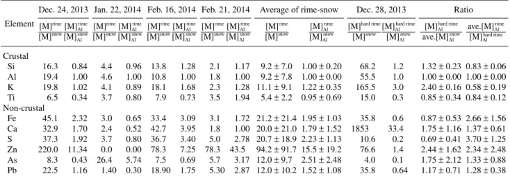
(6) 594. ANALYTICAL SCIENCES MAY 2018, VOL. 34. Table 4 Comparison of elemental ratio of bare component and component normarized by Al of element during one-day meteorological event Dec. 24, 2013 Jan. 22, 2014 Feb. 16, 2014 Feb. 21, 2014 Element [M]rime [M] rime [M]rime [M] rime [M]rime [M] rime [M]rime [M] rime Al Al Al Al [M]snow [M]Alsnow [M]snow [M]Alsnow [M]snow [M]Alsnow [M]snow [M]Alsnow Crustal Si 16.3 Al 19.4 K 19.8 Ti 6.5 Non-crustal Fe 45.1 Ca 32.9 S 37.3 Zn 220.0 As 8.3 Pb 22.5. 0.84 1.00 1.02 0.34. 4.4 4.6 4.1 3.7. 0.96 1.00 0.89 0.80. 13.8 10.8 18.1 7.9. 1.28 1.00 1.68 0.73. 2.32 1.70 1.92 11.34 0.43 1.16. 3.0 2.4 3.7 0.0 26.4 1.40. 0.65 0.52 0.80 0.00 5.74 0.30. 33.4 42.7 36.7 78.3 7.5 18.90. 3.09 3.95 3.40 7.25 0.69 1.75. 2.1 1.8 2.3 3.5. Average of rime-snow rime. [M] [M]snow. 1.17 9.2 ± 7.0 1.00 9.2 ± 7.8 1.28 11.1 ± 9.1 1.94 5.4 ± 2.2. 3.1 1.72 1.8 1.00 5.0 2.78 78.3 43.5 5.7 3.17 5.30 2.87. 21.2 ± 21.4 20.0 ± 21.0 20.7 ± 18.9 94.2 ± 91.7 12.0 ± 9.7 12.0 ± 10.2. rime Al snow Al. [M] [M]. Dec. 28, 2013 hard rime. hard rime Al snow Al. [M] [M] [M]snow [M]. Ratio hard rime Al snow Al. [M] ave.[M]. ave.[M]Alrime [M]Alhard rime. 1.00 ± 0.20 1.00 ± 0.00 1.22 ± 0.35 0.95 ± 0.69. 68.2 55.5 165.5 15.0. 1.2 1.0 3.0 0.3. 1.32 ± 0.23 1.00 ± 0.00 2.40 ± 0.16 0.85 ± 0.34. 0.83 ± 0.06 1.00 ± 0.00 0.58 ± 0.19 0.84 ± 0.12. 1.95 ± 1.03 1.79 ± 1.52 2.23 ± 1.13 15.5 ± 19.2 2.51 ± 2.48 1.52 ± 1.08. 35.8 1853 10.6 76.6 4.0 35.8. 0.6 33.4 0.2 1.4 0.1 0.64. 0.87 ± 0.53 1.75 ± 1.16 0.69 ± 0.41 2.44 ± 1.62 1.75 ± 2.12 1.17 ± 0.71. 2.66 ± 1.56 1.37 ± 0.61 3.70 ± 1.25 2.34 ± 2.48 1.33 ± 0.88 1.28 ± 0.38. Fig. 4 WDXRF data for insoluble substance in snow and rime with standard samples. (A) S-Kα spectrum: a, Na2SO4; b, NaHSO4; c, Na2SO3; d, NaHSO4; e, cystine, f, rime sample at Feb. 21, 2014. (B) Correlation between chemical shift and oxidation number of sulfur. (C) Correlation between chemical shift and fraction of S(VI).. Figure 4(A) shows the WDXRF spectra of standard compounds with different chemical states of elemental sulfur along with that of a rime sample. Low energy shifts of the peaks of the S-Kα line (chemical shift) of the WDXRF spectra indicate reduction of the mean oxidation number. The chemical shifts of the S-Kα line allow the oxidation state of sulfur to be determined by chemical analysis. The calibration graph for the measured oxidation number vs. chemical shift (δ) is shown in Fig. 4(B) as follows: [Observed oxidation number] = –3.00 × δ2 + 2.53 × δ + 5.93. r2 = 0.9965. (19). Plots of the percentage fractions of S(VI) and S(-II) (f [S(VI)]% and f [S(-II)]%) vs. the calculated chemical shift are shown in Fig. 4(C) and the regression curve was: f [S(VI)]% = 13.12 × δ2 + 93.24 × δ + 97.22 r2 = 0.9964,. (20). f [S(-II)]% = 100 – f [S(VI)]%,. (21). where the peak of the S-Kα line was obtained from the synthetic spectrum and was based on weighted averages dependent on the mole fractions..

(7) ANALYTICAL SCIENCES MAY 2018, VOL. 34 Figure 5 shows the δ of various samples of snow, rime, and hard rime. It was observed in this figure that there is no shift in δ in the hard rime sample, indicating the chemical state of the total sulfur species to be S(VI). The reductive atmosphere increased according to the order hard rime < snow < rime  coal combustion emission. The chemical shifts are summarized in Table 5, in which the peak energy for the S-Kα line of Na2SO4 was defined to be zero as the chemical shift standard. The chemical shifts for rime and snow samples that accumulated and were collected within one day (see Table S2) are shown in Table 6 together with that of the coal combustion sample. Additionally, the δ values obtained with high resolution and normal resolution spectra are provided for comparison in Table 6. The δ = –0.018 eV of the hard rime sample was very close to that of the standard S(VI) species (δ = 0.00 eV). The δ for the coal combustion sample obtained using the high resolution mode of WDXRF is consistent within the error of the average δ = –0.819 ± 0.125 eV for the rime samples.. Fig. 5 Chemical shift (δ) of standard sample, coal incomplete combustion emittion, snow, hard rime and rime. Standar samples: S(VI), Na2SO4; S(VI), Na2SO3; S(II), NaHSO4; S(-II), cystine. ○, Average; , ±S.D.. 595 The values of δ = –0.512 ± 0.05 eV for the snow samples analyzed using the normal resolution mode of WDXRF were between the values obtained for the rime and hard rime samples. The observed oxidation state for sulfur estimated using Eq. (19) was found to be 5.88 in the hard rime sample, and nearly equal to that of S(VI). These oxidation states were 1.81 ± 0.90 and 3.84 ± 0.27 in the rime and snow samples, respectively. Thus, the decrease in oxidation state follows the order hard rime < snow < rime  coal combustion emission. It is reasonable to assume that the sulfur compounds found in the insoluble substance were mainly derived from coal combustion and oil combustion, that the average oxidation state of sulfur can be explained by nss-SO4 occurring as an end member of oxidized compounds in the atmospheric layer, and that organic sulfur compounds are produced due to incomplete combustion and burning. The values of f [S(VI)]% and f [S(-II)]% were calculated using Eqs. (20) and (21) and are also shown in Table 6. It was proposed that the S(VI) fraction would be 95.5% in the hard rime sample, 53.0 ± 3.8% in the snow samples, 32.3 ± 8.4% in the rime samples, and approximately 24 – 30% in the incomplete coal combustion emission samples. For the hard rime samples, the δ of the S-Kα line was close to the Na2SO4 standard, indicating that only S(VI) species were present. It is considered reasonable that all the S(VI) species found in the hard rime sample could be from a plaster-like insoluble compound. Figure 6 shows that [crust.-S(VI)]rime can be corrected from [M]rime based on f [S(VI)]hard rime = 0.955, [S]hard rime/[Ca]hard rime = 0.3567, [S]hard rime/[Si]hard rime = 2.548 × 10–3, and [S]hard rime/[Al]hard rime = 6.379 × 10–3: [crust.-S(VI)M]rime= f [S(VI)]hard rime × ([S]hard rime/[M]hard rime) × [M]rime,. (22). [crust.-S(VI)Ca]rime= 0.955 × 0.3567 × [Ca]rime,. (23). [crust.-S(VI)Si]rime= 0.955 × 2.548 × 10–3 × [Si]rime,. (24). [crust.-S(VI)Al]rime= 0.955 × 6.379 × 10–3 × [Al]rime.. (25). The value of [n.c.-S(-II)]rime was estimated using the equation: [n.c.-S(-II)M]rime= [S]rime – [crust.-S(VI)M]rime.. (26). Table 5 X-Ray spectral chemical shift (δ) of the S-Kα peak in standard sustrates δ, eV S(VI) This work. Kavcˇicˇ26. Wenqi27. Ito28. Na2SO4 0.00 NaHSO4 0 (NH4)2SO4 0.00 ± 0.04 Fe2(SO4)3 –0.04 ± 0.04 Inorg.-S(VI) 0.000 – +0.020 Org.-S(VI) –0.153 – –0.323 NaHSO4 0.00. S(IV). S(II). Na2SO3 –0.44 NaHSO3 –0.44 Na2SO3 –0.42 ± 0.04. Na2S2O3 –0.83. S(IV) –0.386. S(0) –1.195. NaHSO3 –0.37 HOCH2SO2Na·2H2O –0.3. HOCH2SO2Na·2H2O –0.56. S(0). S(-II) Cystine –1.25 TiS –1.35 ± 0.04 FeS –1.37 ± 0.04 Inorg.-S′(-II) –1.202 – –1.301 Org.-S(-II) –1.371 – –1.411. Sulfur –1.12.

(8) 596. ANALYTICAL SCIENCES MAY 2018, VOL. 34. Table 6 Mole fraction in percent (%) of S(VI) and S(-II) calculated by the chemical shift (δ) of S-Kα line in hard rime, rime, and snow at No. 1 site with coal combution exhaust substance Sample. Date. Mode. δ/eV. Oxidation state S(X). obs.. Coal burining exhaust substance Hard rime Rime. Snow. Dec. 28, 2013 Dec. 24, 2013 Jan. 22, 2014 Feb. 16, 2014 Feb. 21, 2014 Average Dec. 24, 2013 Jan. 22, 2014 Feb. 16, 2014 Feb. 21, 2014 Average. Ha Nb N H H H H N H N N H N N H N. –0.802 –0.896 –0.018 –0.828 –0.818 –0.618 –0.872 –0.900 –0.819 ± 0.125 –0.486 –0.548 –0.548 –0.555 –0.458 –0.420 –0.512 ± 0.05. 1.97 1.25 5.88 1.78 1.85 3.22 1.44 1.22 1.81 ± 0.90 3.99 3.64 3.64 3.60 4.14 4.34 3.84 ± 0.27. Fraction S(VI), %. S(-II), %. 30.9 24.2 95.5 29.0 29.7 44.6 25.9 23.9 32.3 ± 8.4 55.0 50.1 50.1 49.5 57.3 60.4 53.0 ± 3.8. 69.1 75.8 4.5 71.0 70.3 55.4 74.1 76.1 67.7 ± 8.4 45.0 49.9 49.9 50.5 42.7 36.9 47.0 ± 3.8. a. H is a high resolution spectra. b. N is a normal resolution spectra.. Fig. 6 Plots of [M] vs. [S] in rime and snow collected on the one-day accumulation in Table 6. (A) Ca; (B) Si; (C) Al. Solid line is a ratio of [obs.M] vs. [obs.S] in the hard rime. ●, Snow; ▲, rime; △, hard rime at No. 1 site. ○, Snow at various sites in Japan.. The values of f [crust.-S(VI)M]rime% and f [n.c.-S(-II)M]rime% are defined as: f [crust.-S(VI)M]rime% = [crust.-S(VI)M]rime/[S]rime × 100 = fS(-II)crustal,. (27). f [n.c.-S(-II)M]rime% = [n.c.-S(-II)M]rime/[S]rime × 100 = fS(-II)crustal. (28). The observed values are shown in Table 7. The [crust.-S(VI)Ca]rime% values are close to that based on the δ and their averages are in agreement within the standard deviation. The average values of f [crust.-S(VI)Si]rime and f [crust.-S(VI)Al]rime% were significantly about 10% lower than that of f [crust.-S(VI)Ca]rime%. The plotted points of some snow samples occurred below the regression line of hard rime (Figs. 6(B) and 6(C)). Equation (23) is more reliable than the Eqs. (24) and (25)..

(9) ANALYTICAL SCIENCES MAY 2018, VOL. 34. 597. Table 7 Mole fraction in percent (%) of S(VI) and S(-II) based on the [M] in hard rime at No. 1 site Date Dec. 24, 2013 Jan. 22, 2014 Feb. 16, 2014 Feb. 21, 2014 Average ± SD. Ca. Si. Al. S(VI), %. S(-II), %. S(VI), %. S(-II), %. S(VI), %. S(-II), %. 38.0 28.6 42.1 29.5 34.6 ± 6.4. 62.0 71.4 58.0 70.5 65.5 ± 6.5. 14.2 29.0 24.8 24.6 23.2 ± 6.3. 85.8 71.0 75.2 75.4 76.9 ± 6.3. 17.5 37.6 29.2 27.3 27.9 ± 8.3. 82.5 62.4 70.8 72.7 72.1 ± 8.3. Fig. 7 Fraction of S(VI) and S(-II) of insoluble sulfur with their content classified by back trajectry , fraction of S(VI); , S(-II); ○, observed [S]. of air mass.. Figure 7 shows f [crust.-S(VI)Ca]snow and f [n.c.-S(-II)Ca]snow% estimated using Eq. (23). The fraction of S(-II) decreased from 92 to 57% from the Chugoku district (Nos. 3, 4 and 5) to the Shikoku district (No. 1), which would lead to the selective deposition of S(-II) species with no relation to [S]snow. After snowfall in the Chugoku district, snowfall occurred again when the cold air mass reached the Shikoku district. Since larger airborne particulate matter and dust are more easily deposited than smaller particles, the fraction of smaller particles would increase. The size of carbonaceous substances containing the S(-II) form is larger than that of the sulfate aerosols. The f [n.c.-S(-II)Ca]snow% was 66% in the Kinki district (No. 7), 24% in the Hokuriku district (Nos. 8 and 10), and 31% in the Tohoku district (No. 11). The snowfall in the Hokuriku and Tohoku districts is significantly larger than that in the Kinki district. Thus, the value of f [S(-II)Ca]snow% for the Hokuriku and Tohoku districts should be lower than that of the Kinki district. Figure 7 clearly shows a tendency for the fraction of S(-II) to decrease from west Japan to northeast Japan independently of whether the air mass origins were Dongbei, China, or Russia. It is important to consider the amount of insoluble sulfur that it is commonly found in Japan, and therefore snow samples collected in clean remote areas can be observed for Nos. 4, 9, and 12. Less insoluble sulfur (below the LOD) is deposited after the remaining cold air masses around the Japan islands have ceased for at least 24 h following a snowfall event near the coast of the Japan Sea, as evidenced by where the Kinki-Shikoku (Dec. 30, 2015 at No. 4), the Kanto-Chubu (Feb. 8, 2014 at No. 9), and. the Tohoku area (Feb. 4, 2015 at No. 12) samples were collected. This fact indicates that there is a trivial amount of insoluble sulfur compounds contained in the cold air masses at relatively high altitudes in Japan. During the one-day meteorological event involving rime and snow, it can be assumed that the components in its cold air mass area are nearly constant because the meteorological conditions are the same as at the rural clean area of No. 1 site with a high altitude of 1400 m. The insoluble substrate of rime ice contains smaller-sized snow-like condensation nuclei and larger substances deposited by inertial collisions. The S(-II) species should be contained in both the snow-like component and the inertial condensation component. The value of δ provides the fraction of S(-II) in whole rime (f[S(-II)]rime) and in snow (f[S(-II)]snow), which corresponds to the snow-like component in the rime. Currently, there is no information about the fraction of S(-II) in substrates deposited by inertial collisions (f[S(-II)]collision). [S]rime × f[S(-II)]rime = [S(-II)]rime = [s.o.-S]rime × f[S(-II)]snow+ [ex.S]rime × f[S(-II)]collision,. (29). where f[S(-II)]rime (= f [S(-II)]rime%/100) and f[S(-II)]snow (= f [S(-II)]snow%/100) are shown in Table 6. The values of [s.o.-S]rime and [ex.S]rime were obtained using Eqs. (15) and (16) (shown in Table S2). Since [S]rime is an observed value, the unknown parameter (f[S(-II)]collision) can be calculated. Table 8 shows the value of f[S(-II)]collision obtained. The f[S(-II)]collision values were 78, 85, and 81%, which were higher than f[S(-II)]snow on Dec. 24, 2013;.

(10) 598. ANALYTICAL SCIENCES MAY 2018, VOL. 34. Table 8 Mole fraction in percent (%) of the S(VI) and S(-II) species in non-crustal sulfur in the rime at No. 1 site Date Dec. 24, 2013 Jan. 22, 2014 Feb. 16, 2014 Feb. 21, 2014 Average. 6.. Fraction, % S(VI). S(-II). 22.0 15.0 41.8 18.8 22.4 ± 11.6. 78.0 85.0 58.2 81.2 75.6 ± 11.6. 7. 8. 9. 10. 11.. Jan. 22, 2014; and Feb. 21, 2014. The value of f[S(-II)]collision was 76 ± 12% from the average content, which was close to that obtained from the combustion origin.. Conclusions It can be concluded that speciation of the insoluble S species in a wet deposition in the winter could be estimated from the chemical shift of the S-Kα line, and that the WDXRF technique should be capable of determining the fractionation, f[S(VI)]rime and f[S(-II)]rime, using only [S]rime and [Ca]rime. The SEM images clearly demonstrate deposition by the inertial collision of larger particulates during exposure to cold air flow of the winter monsoon. Comparing the components of snow, rime, and hard rime samples obtained during the one day meteorological event with similar meteorological factors showed that the advantage of the textured surface morphology of rime ice is due to the scavenging of aerosol particles by inertial collisions, particularly the low oxidation state form of insoluble sulfur species produced by the incomplete combustion of coal. Low oxidation state sulfur would be contained in urban dust and/or airborne particulate matter.. Acknowledgements. 12. 13. 14. 15. 16. 17. 18. 19. 20. 21. 22. 23. 24.. JSPS KAKENHI Grant No. 26340084 supported this work. We would like to thank the Hitachi High-Technologies Co., Ltd. for SEM observation.. 25. 26.. Supporting Information. 27.. This material is available free of charge on the Web at http:// www.jsac.or.jp/analsci/.. 28. 29.. References 30. 1. S. Tsunogai and T. Shinagawa, Geochem. Soc. Jpn., 1997, 11, 1. 2. H. Mukai, Y. Ambe, T. Muku, K. Takeshita, T. Fukuma, J. Takahashi, and S. Mizota, Res. Rep. Natl. Inst. Environ. Stud., Jpn., 1989, 123, 7. 3. Y. Sekine and Y. Hashimoto, J. Jpn. Soc. Air Pollut., 1991, 26, 216. 4. D. Zhao, J. Xiong, Y. Xu, and W. Chan, Atmos. Environ., 1988, 22, 349. 5. X.-Y. Yang, Y. Okada, N. Tang, S. Matsunaga, K. Tamura,. 31. 32. 33. 34.. J.-M. Lin, T. Kameda, A. Toriba, and K. Hayakawa, Atmos. Environ., 2007, 41, 2710. R. Motoyama, F. Yanagisawa, N. Akata, Y. Suzuki, Y. Kanai, T. Kojima, A. Kawabata, A. Ueda, A. Kawabata, and A. Ueda, Seppyou, 2002, 64, 49. N. Akata, F. Yanagisawa, R. Motoyama, A. Kawabata, and A. Ueda, Seppyou, 2002, 64, 173. H. Mukai, A. Tanaka, and T. Fujii, J. Jpn. Soc. Atmos. Environ., 1999, 34, 86. L. X. Zhong and Y.-S. Chung, Atmos. Environ., 1996, 30, 2355. S. Itabashi, H. Hayami, J. Jpn. Soc. Atmos. Environ., 2015, 50, 138. T. Tanabe, Y. Tanaka, D. Tanaka, Y. Taniguchi, M. Toyoda, J. Kawai, H. Ishii, C. Riu, Y. Yilixiati, S. Hayakawa, Y. Kitajima, and Y. Terada, Bunseki Kagaku, 2004, 53, 1411. Y. Ban, I. Watanabe, K. Furuya, H. Matsushita, and Y. Gohshi, Bunseki Kagaku, 1985, 34, 264. Y. Ban, K. Furuya, T. Kikuchi, A.-P. Wan, Y.-C. Huang, C.G. Ma, and J. Wu, J. Jpn. Soc. Air Pollut., 1985, 20, 470. W. H. Calkins, Energy Fuels, 1981, 1, 59. Z. Shi, L. Shao, T. P. Jones, A. G. Whittaker, S. Lu, K. A. Bérubéc, T. He, and R. J. Richards, Atmos. Environ., 2003, 37, 4097. S. Imai, Y. Yamamoto, Y. Sanagawa, Y. Kurumi, I. Kurotani, J. Nishimoto, and Y. Kikuchi, Bunseki Kagaku, 2017, 66, 95. Y. Sanagawa, Y. Kurumi, Y. Yamamoto, T. Kamimura, and S. Imai, Bunseki Kagaku, 2014, 63, 351. Y. Kurumi, Y. Sanagawa, Y. Yamamoto, T. Kamimura, and S. Imai, Bunseki Kagaku, 2014, 63, 837. S. Imai, Y. Yamamoto, and T. Kamimura, Bunseki Kagaku, 2016, 65, 211. G. P. Huffman, S. Mitra, F. E. Huggins, N. Shah, S. Vaidya, and F. Lu, Energy Fuels, 1991, 5, 574. R. G. Hurly and E. W. White, Anal. Chem., 1974, 46, 2234. L. S. Brirks and J. V. Gilfrich, Spectrochim. Acta, Part B, 1978, 33, 305. E. Martins and D. S. Urch, Anal. Chim. Acta, 1994, 286, 411. Y. Gohshi, O. Hirao and I. Suzuki, Adv. X-ray Anal., 1975, 18, 406. S. Matsumoto, Y. Tanaka, H. Ishii, T. Tanabe, Y. Kitajima, and J. Kawai, Spectrochim. Acta, Part B, 2006, 61, 991. M. Kavc´ic´, A. G. Kraydas, and C. Zarkadas, X-ray Spectrom., 2005, 34, 310. W. Qi, J. Kawai, S. Fukushima, A. Iida, K. Furuya, and Y. Gohshi, Bunseki Kagaku, 1987, 36, 301. H. Itoh, Y. Takahashi, A. Fukushima, and Y. Gohshi, Adv. X-ray Anal., 1989, 20, 59. S. Gao, T.-C. Luo, B.-R. Zhang, H.-F. Zhang, Y.-W. Han, Z.-D. Zhao, and Y. K. Hu, Geochim. Cosmochim. Acta, 1998, 62, 1959. T. Narukawa, A. Takatsu, K. Chiba, K. W. Riley, and D. H. French, J. Environ. Monit., 2005, 7, 1342. Meteorological Data Explorer, Centre for Global Environmental Research (CGER-METEX ), http://db.cger. nies.go.jp/metex/index.html. C.-L. Chau, Int. J. Coal Geol., 2012, 100, 1. K. Sugawara, T. Gunji, and T. Sugawara, Energy Fuels, 1997, 11, 1272. K. Sugawara, Y. Enda, T. Kato, T. Sugawara, and M. Shirai, Energy Fuels, 2003, 17, 204..

(11)