© JCRM All rights reserved.
Volume 10, Number 1, October 2014, pp.5-14
[Issue paper]
A method for measurement of rock stress change - Cross-sectional borehole deformation method -
Yuzo OBARA*, Toru YOSHINAGA**, Minami KATAOKA* & Tatsuya YOKOYAMA***
* Member of ISRM: Graduate School of Science and Technology, Kumamoto University, Chuo-ku, Kumamoto 860-8555 Japan
** Member of ISRM: Faculty of Engineering, Kumamoto University, Chuo-ku, Kumamoto 860-8555 Japan
*** Member of ISRM: Energy Division, OYO Co. Ltd., Minami-ku, Saitama, 336-0015, Japan Received 08 04 2014; accepted 05 09 2014
ABSTRACT
A method for measurement of stress change is suggested to monitor rock stress using a borehole. The two-dimensional state of stress change in a plane perpendicular to the axis of a borehole drilled within a rock mass can be measured by this method, which is named the Cross-sectional Borehole Deformation Method (CBDM). In this paper, the theory of the CBDM is firstly described, as well as the prototype instrument and theoretical procedure for correcting eccentric positioning of the instrument in the borehole.
Then the estimation of the stress change is demonstrated in a laboratory experiment, using a granite plate with a borehole. Finally, applying the CBDM to measured stress change around an underground cavern during and after excavation, the changes of rock stress distribution around the cavern is shown. It makes clear that stress change in the immediate rock mass of the cavern can be estimated by the CBDM and that the CBDM is available for measuring rock stress change.
Keywords: Rock stress measurement, Stress change, Cross-sectional Borehole Deformation Method (CBDM), In-situ Measurement
1. INTRODUCTION
Knowledge of rock stresses, such as initial stress and induced stress, is of fundamental importance for designing and constructing rock structures. In order to measure initial stress, many methods have been suggested. On the other hand, there are some methods for stress change around an opening under construction. For example, the stress change of an underground power house has been measured by a vibrating wire strain gauge in Japan (Kudo et al. 1998). However, using this gauge, the stress in only one direction in a plane perpendicular to a borehole axis is measured.
The Cross-sectional Borehole Deformation Method (CBDM) developed by Taniguchi et al. (2003) and Obara et al. (2004, 2010, 2011a, b, 2012 a, b) is a method by which the two-dimensional state of stress change within a rock mass in a plane perpendicular to a borehole axis can be measured.
Kiguchi and Kuwahara (2013) and Kawabe et al. (2005) have developed instruments having the same concept of the authors. The instrument suggested by Kiguchi et al. was installed in a vertical borehole with a diameter of more than 100mm just after drilling, then the change of the cross-sectional shape of the borehole was measured by a laser displacement sensor with a resolution of 0.7m. They estimated only orientation of principal directions in the horizontal plane without magnitude of principal stresses. On
the other hand, the instrument developed by Kawabe et al.
was installed in a borehole with a diameter of 76 to 100mm.
The laser displacement sensor which was used has a measurement range of 30 to 50mm with a resolution of 2m.
This resolution is insufficient for measuring displacement of hard rock due to small stress changes. In this method, they tried to estimate the stress state in the perpendicular of a borehole axis in a laboratory experiment. However, they did not discuss the evaluated result in the case that the axes of the borehole and the instrument did not coincide with each other – namely, an eccentric position of the instrument. This coincidence of both axes is an important factor to obtain the displacement distribution and shape of a cross-section of the borehole with a high accuracy. However, they did not treat this problem. Berard and Cornet (2003) suggested the method of correction of eccentric positioning of a borehole televiewer tool to obtain the shape of a borehole cross-section for estimating borehole breakout. In the CBDM, a non-linear programming for optimization with the non-linear least square method is introduced into the correction method to solve the eccentric position of the instrument.
In this paper, the CBDM is introduced to measure rock stress change in laboratory and in-situ experiments. Firstly, the developed prototype instrument used in the CBDM is described, as well as the theory of the CBDM. In order to estimate the displacement distribution of a cross-section of the borehole precisely, both axes of the borehole and the
instrument must coincide with each other. However, it is difficult to coincide physically. Therefore, a theoretical procedure for coinciding with both axes of the borehole and the instrument, namely correcting eccentric positioning of the instrument, is introduced to the method. Then the estimation of the stress change which acted on the granite plate with a borehole is demonstrated in the laboratory experiment.
Finally, applying the CBDM to measured stress change around an underground cavern during and after excavation, the changes of rock stress distribution around the cavern is shown. It makes clear that stress change of immediate the rock mass of the cavern can be estimated by the CBDM and that the CBDM is available for measuring rock stress change.
2. OUTLINE OF CBDM
2.1 Measurement of displacement on borehole wall and Instrument
The rock mass around a borehole is elastically deformed corresponding to subjected rock stress. Based on this principle, a method was developed for easily and accurately measuring two-dimensional stress change in a plane perpendicular to the borehole axis. This method is the Cross-sectional Borehole Deformation Method (CBDM). The displacement of the borehole wall is measured by a non-contact typed sensor, namely a laser displacement sensor, which is inserted and rotated in the borehole as shown in Figure 1. Accordingly, the rigidity of the instrument becomes
zero for the measurement, because the displacement of the borehole wall can be measured without touching the wall.
Then the rock mass around the borehole is undisturbed due to measurement, such as the hydraulic fracturing method.
In order to measure radial displacement of the wall in a cross-section of the borehole, a compact and accurate laser displacement sensor is used. The dimensions are 43mm×
40mm×18mm, and the resolution is 0.1 m. A small stepping motor is adopted for rotation of the laser displacement sensor. The minimum angle of rotation step of the stepping motor is 0.1 degrees.
(b) (c) (d)
(a)
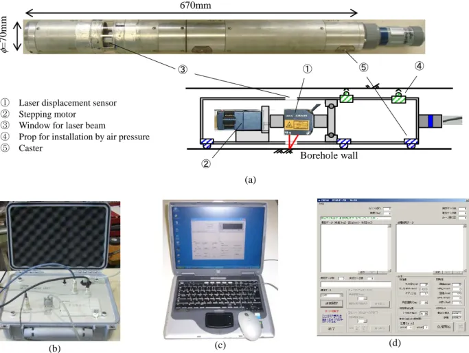
① Laser displacement sensor
② Stepping motor
③ Window for laser beam
④ Prop for installation by air pressure
⑤ Caster
670mm
=70mm
②
③ ① ⑤ ④
Borehole wall
Figure 2. Schematic view of prototype instrument and devices for control of instrument; (a) prototype instrument, (b) control box, (c) PC and display, (d) example of display of program.
Figure 1. Principle of measuring displacement of a borehole wall.
X Y
Deformed borehole
Borehole of True round
Laser displacement sensor
Laser reflection
X Y
Deformed borehole
Borehole of True round
Laser displacement sensor
Laser reflection Laser displacement sensor
Deformed borehole
Laser beam
Drilled borehole
The prototype instrument for measurement and schematic view are shown in Figure 2. The tube of the instrument, 70 mm in diameter and 670 mm in length, is aluminum. The instrument is fixed in a borehole using two air pistons. The laser displacement sensor is located near small windows which are covered by acrylic plates for waterproof, and rotated by the stepping motor set in a head of the instrument.
The motor is controlled by a computer through a controller and a driver. On the other hand, the output from the laser displacement sensor is stored in a computer through an amplifier unit and a data logger. These are assembled into the control box as shown in Figure 2(b). The sensor and motor are linked by the cables of about 30m length (Obara et al.
2012a).
2.2 Principle of measurement
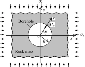
The schematic view of a cross-section in a plane perpendicular to the borehole axis is shown in Figure 3. The borehole having a cross-section of perfectly circular is drilled within a rock mass. Its radius is defined by R. The homogeneous and isotropic rock mass is assumed to be infinite and elastic. The principal stress subjected at infinity is defined in the x-y coordinate system which is set on the borehole with the origin at its axis in Figure 4:
{} = {x, y} (1) The axes in the coordinate system coincide with the principal directions.
The radial displacements due to each principal stress are described as:
) 2 cos 2 1 )(
1 (
), 2 cos 2 1 )(
1 (
2 2
E U R
E U R
y y R
x x R
(2)
In general, the radial displacement UR is the vector sum of displacement UR x and UR y, which are generated corresponding to each principal stress (Jaegar & Cook 1979):
(x y) 2(x y)cos2
y R x R
R U U H
U (3)
where H = R(1-2)/E, E is Young’s modulus and is Poisson’s ratio, then is rotation angle with the positive x axis. The radius RR after deformation is represented:
RR=R+UR (4) In a measurement, the displacements and measured radii, number of n, are denoted by:
{UR} = {UR1, UR2, …., URi, …., URn} (5) {RR} = {RR1, RR2, …., RRi, …., RRn}
The coordinates of the measuring point i on the borehole wall are written in the X-Y coordinate system defined on the instrument with the origin at its axis in Figure 4 as follows:
Xi = RRi cosYi = RRi sin(6) where is the rotation angle with the positive X axis in Figure 4. The measured results schematically are shown in this figure. The plots represent measurement values, and the solid curve is approximately expressed by an ellipse with a center of (0, 0) in x-y and (b, d) in an X-Y coordinate system.
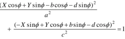
The length of major and minor axes of the ellipse is 2a and 2c, respectively. In general, the center of the ellipse does not coincide with that of the borehole as shown in the figure. In the cases that the distance between origins of each center is very short, the equation of the ellipse in the x-y coordinate system may be written as:
(7) Using the coordinate transformation law from the X-Y to x-y coordinate system represented by eq(8), the observation equations are obtained at each measurement point as eq(9).
cos ) ( sin ) (
, sin ) ( cos ) (
d Y b
X y
d Y b
X x
(8)
2 1
2 2
2
c y a x
Figure 3. Schematic view of cross section of a borehole drilled within rock mass, which is assumed to be infinite and elastic.
y y
R Borehole
Rock mass
o x x
UR
r
y y
R Borehole
Rock mass
o x x
UR
r
Figure 4. Schematic diagram of measured results and approximated ellipse by a non-linear least square method.
X and Y axes are defined on an instrument, then x and y axes defined on a borehole coincide with principal direction.
Major axis
a
o
c
Y
y
x
X
Measured Approximated (b,d)
Minor axis
) 1 cos sin cos sin (
) sin cos sin cos (
2
2 2
2
c
d b Y X
a
d b Y X
(9)
The most probable parameters of an ellipse, a, c, b, d, , are determined by applying a non-linear least square method to observation equations for measured values. When the axis of the instrument coincides with that of the borehole, the parameters b and d are equal to zero.
The displacements on major and minor axes of the determined ellipse are:
(10) Accordingly, most probable principal stresses can be obtained in the x-y coordinate system as follows:
H R c a H
R c a
y
x 8
4 , 3
8 4
3
(11)
Then the stress components in the X-Y coordinate system are calculated by the stress transformation law.
The stress estimated from eq(11) is not correct, because it is impossible to measure the radius of the borehole precisely just after boring (Obara et al., 2010). Therefore, the absolute stress state cannot be estimated. The stress determined by eq(11) is considered to be a temporal stress.
The stress change can be estimated, using the temporal stress at more than two stages as follows. For example, the state of stress is changed with progress of construction of the underground opening. At the first stage, a borehole is drilled within a rock mass, and the cross-sectional shape of the borehole is measured at an early stage of excavation of an opening. Using the displacement, the temporal stress at the first stage can be determined. At the second stage, the shape at the same section of the borehole is measured again and the temporal stress is determined at an arbitrary stage during excavation. Then, the stress change is determined by the difference of temporal rock stress states determined at the first and second stages of excavation, assuming that rock is elasti. Thus, the stress change due to elapsed time or excavation can be estimated by measuring the cross-sectional shape at the same cross-section of one borehole repeatedly.
Consequently, the temporal stress state {I}={XI, YI, XYI} is assumed at the first stage. The temporal stress {II}={XII,
YII, XYII} is also assumed at the second stage. The stress change {} can be estimated by the following equation, using the estimated temporal stress state at two stages:
{} = {X, Y, XY}={II}{I} (12)
3. THEORETICAL ANALYSIS OF INFLUENCE FACTORS ON MEASUREMENT RESULTS
According to parameter H in eq(3), the estimated stress is a function of borehole radius, Young’s modulus, and Poisson’s ratio of rock. Eq(7) is the observation equation in cases that the distance between axes of the borehole and the instrument is very short. If that distance becomes longer, namely, by eccentric positioning of the instrument, the estimated stress is also influenced by the distance. In this chapter, the influence of borehole radius, Young’s modulus,
and distance between both axes in the estimated result is discussed under a condition of =0.2, because that the influence of Poisson’s ratio is smaller, comparing with the above parameters.
3.1 Borehole radius
The three cases of principal stress state are assumed under condition of R=38mm and E=30GPa as follows; I) {I} = {xI, yI} = {5, 10}, II) {II} = {5, 15}, III) {III} = {5, 30}
(unit: MPa). The distribution of displacements UR of a borehole wall is calculated in the case of R=38mm by eq(2).
Then the radius distribution RR in eq(4) is calculated by eq(3).
Assuming that the calculated RR is the measured one, the )
3 ( ),
3
( x y c R H y x
H R
a
-0.2 -0.1 0 0.1 0.2
0 45 90 135 180 225 270 315 360
Displacement , mm
, degree
R=37.90mm
38.00mm
38.10mm
0 10 20 30 40 50
37.88 37.92 37.96 38.00 38.04 38.08 38.12 Radius of borehole, mm
Estimated stress change, MPa
y=20MPa
y=5MPa
y=10MPa 0
10 20 30 40 50
37.88 37.92 37.96 38.00 38.04 38.08 38.12
Estimated principal stress, MPa
Radius of borehole, mm
y=30MPa
y=10MPa
y=15MPa
Figure 5. Influence of borehole radius on estimation of initial stress and stress change; (a) distribution of displacement of borehole wall, (b) estimated initial stress y, (c) estimated stress change y.
(a)
(b)
(c)
distribution of displacement can be calculated under a different radius as shown in Figure 5(a), in the cases that the axis of the borehole coincides with that of the instrument.
All distributions of displacement in the case of a different radius have a period of and the same amplitude. However, each magnitude is dependent on the assumed radius.
Using these displacements, the most probable stress is estimated by the non-linear least square method as shown in Figure 5(b). The estimated stress y is represented with the assumed radius. The black circles in the figure represent the real stress value in the case of R=38mm. The stress increases with increasing radius. If the radius can be measured with a high accuracy, the initial stress is determined. However, it is impossible to measure borehole radius precisely.
Consequently, initial stress cannot be estimated by the CBDM.
Considering the stress change of stages I) to II), II) to III) and I) to III), the stress changes y are 5, 10 and 20MPa theoretically. The estimated stress change is shown in Figure 5(c) with various radii. It is clear that the stress change is independent of borehole radius. The stress change can be estimated even if the radius is not measured with a high accuracy.
The stress state is a temporary stress state, and the stress change is real stress. Accordingly, the CBDM is available for estimating stress change.
3.2 Young’s modulus
The distribution of displacement of a borehole wall is calculated by eq(3) under the condition of R=38mm and E=30GPa. Using these displacements, the most probable stress is estimated by the non-linear least square method.
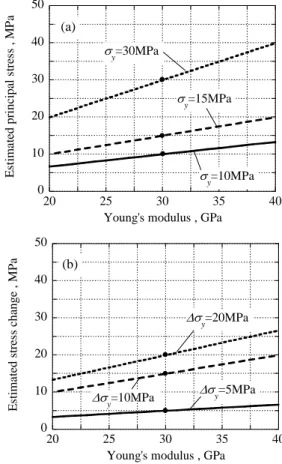
Figure 6(a) and (b) show estimated stress y and y with various Young’s moduli. Both stress and stress change are proportional to Young’s modulus. The degree of proportion is dependent on the magnitude of stress. The influence of Young’s modulus on measurement result in stress and stress change is almost the same in conventional stress measurement methods based on the theory of elasticity.
Therefore, precise estimation of Young’s modulus is also important to estimate stress change by the CBDM.
3.3 Installation position of instrument in a borehole
In the measurement, the instrument is inserted into a borehole. The axis of the instrument does not usually coincide with that of the borehole, that is, the instrument is installed at an eccentric position to the center of a cross-section of the borehole. The coordinate systems are defined as shown in Figure 7. The X’-Y’ coordinate system is defined in the instrument, as its origin o’ is the axis of the instrument, then the X-Y and x-y coordinate systems are defined in the borehole, as its origin o is the axis of the borehole. The axes of X’ and X in the coordinate systems are parallel. The coordinates of the origin o are (X, Y) in the X’-Y’
coordinate system.
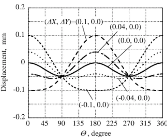
Figure 8 shows the distributions of displacement of a borehole wall in a case that the axis of the borehole is located at X=0, ±0.04 and ±0.1mm with Y=0mm under the condition of R=38mm and E=30GPa. When the distance of both axes is zero, the distribution has a period of and the most probable stress may be estimated by the non-linear least
square method. However, with an increase in the distance, a period of 2is seen in the distribution.
The distribution of the displacement uM is shown as opened plots in the case of X=0mm, Y = 0.1mm in Figure 9. The distribution has a period of 2Applying the non-linear least square method to the distribution of placement, which is assumed to be the measured distribution uM, the approximated curve uA is obtained in Figure 9. The measured data was calculated under assumption of eccentric positioning of the instrument and zero in displacement at
=0. Since the curve is incorrect, it is impossible to estimate the most probable stress by only the non-linear least square method using eq(7).
0 10 20 30 40 50
20 25 30 35 40
Estimated principal stress , MPa
Young's modulus , GPa
y=30MPa
y=10MPa
y=15MPa
Figure 6. Influence of Young’s modulus on estimation of initial stress and stress change; (a) estimated initial stress, (b) estimated stress change.
0 10 20 30 40 50
20 25 30 35 40
Estimated stress change , MPa
Young's modulus , GPa
y=20MPa
y=5MPa
y=10MPa
o’
o
X’
Y’ x
Y
X y
X Y
a c
Figure 7. Definition of coordinate system (a)
(b)
In order to resolve this problem, namely, to correct eccentric positioning of the instrument, a non-linear programming for optimization is introduced into the correction method. The error function fbetween the estimated displacements by the non-linear least square method and measured ones is defined as:
(13)
where n is the number of data. An example of the error function is shown in Figure 10. The shape of that is monotonically decreasing function and unimodal function which has minimum value at the origin. Therefore, this error function can be minimized by a non-linear programming for optimization, moving the origin of the X-Y coordinate system.
The technique of golden section search is introduced in the non-linear programming for finding the minimum of the function. The technique derives its name from the fact that the algorithm maintains the function values for triples of points whose distances form a golden ratio. In the programming, firstly a certain Y0 is given, then the minimum of the function is found in the plane of Y’ =Y0 by golden section research and X0 is obtained at the same time.
The optimized coordinate Y1 is obtained in the plane of X’
=X0 by golden section research. Then, the coordinate X1 is searched for in the plane of Y’ =Y1. This procedure is iterated until the coordinates converge on the constant value (X, Y). The condition of convergence is defined as:
(14)
where i is the iteration number. In the following analysis, || is equal to 10-5mm. After the analysis, we can obtain the temporary stress components on the X-Y and x-y coordinate system, as well as (X, Y).
As examples, three theoretical distributions of displacement of a borehole wall on the X’-Y’ coordinate system are calculated in Figure 11 as a solid line under the condition that {} = {x, y} = {5, 15} (unit: MPa), R=38mm, E=30GPa and =0.2. The rotation angle is zero in Figure 11(a), (b) and 15 degrees in Figure 11(c). In these cases, the axis of the instrument coincides with that of the borehole.
On the other hand, the distribution of displacement represented by the solid line is changed to the opened plots in the case that the distance between both origins of the coordinate systems is large as follows:
Case A : (X, Y)=(-0.2, 0.0) , = 0 in Figure 11(a) Case B: (X, Y)=(0.0, -0.6) , = 0 in Figure 11(b) Case C: (X, Y)=(0.8, 0.4) , =15 degrees in Figure 11(c) The distributions of the plots begin to have a period of 2.
The distribution in each case is perfectly different from the solid line in the case of a coincidence of both axes
Assuming that these distributions are the measured ones, the most probable stress state is calculated on the X-Y and x-y coordinate system, using the developed no-linear programming with the non-linear least square method. The results are summarized in Table 1. The X and Y are described down to the third decimal place and coincide with the given condition of calculation. The constants b to d are those in eq(8). Both b and d are less than 10-4mm. This means that the origin of the X-Y coordinate system coincides with that of the X’-Y’ coordinate system and that the eccentric position of the instrument is perfectly corrected.
Since the radius of the borehole and Young’s modulus are known in this calculation, the stress state is estimated precisely. However, the stress state is a temporary one in the
) , ...
, 1 ( )
( 2
n n i
u u f
n i
i A i
M
i i i
i ΔX and ΔY ΔY
ΔX
1 1
-0.2 -0.1 0 0.1 0.2
0 45 90 135 180 225 270 315 360
Displacement, mm
, degree (X, Y)=(0.1, 0.0)
(0.04, 0.0) (0.0, 0.0)
(-0.04, 0.0) (-0.1, 0.0)
Figure 8. Theoretical distribution of displacement in the case of eccentric positioning of the instrument.
Figure 9. Approximated ellipse curve by a non-linear least square method, based on the measured distribution of displacement.
-0.2 -0.1 0 0.1
0 45 90 135 180 225 270 315 360
Displacement, mm
, degree
Measured data : Approximated curve : uA
uM
Figure 10. Shape of error function of the difference between approximated distribution of displacement and measured one.
0 0.002 0.004 0.006 0.008
Y, mm
X, mm f
cases that the radius of a borehole is unknown. Its principal stress and principal direction is in agreement with the input data. Accordingly, it is concluded that the temporary stress state can be measured by the developed programming, and that stress change can be estimated by the CBDM.
4. LABORATORY EXPERIMENT
The granite plate of 400mm×400mm×47mm with a borehole having a radius of 37.9mm is vertically loaded by a material testing machine as shown in Figure 12. Young’s modulus and Poisson’s ratio of granite are 30 GPa and 0.2, respectively. The X-Y coordinate system is defined on the plate. The vertical stress SY is applied 3 MPa to 5 MPa, and SX is zero. The stress changes Y =2MP is estimated as the
difference from the temporal stresses at two loading stages.
The displacement of the borehole under the condition of SY = 3 and 5 MPa are shown in Figure 13. The closed plots represent the measured displacement. The opened plots are the corrected data for eccentric positioning of the instrument and the solid line is the approximated curve. The corrected data is in agreement with the approximated distribution.
The temporal stress and stress change are estimated in the X-Y coordinate system. The results are summarized in Table 2.
-1 0 1
0 45 90 135 180 225 270 315 360
Displacement, mm
, degree Measured
Theoretical -1
0 1
Displacement, mm Measured
Theoretical -1
0 1
Displacement, mm Measured
Theoretical (a)
(b)
(c)
Figure 11. Distribution of theoretical and measured displacement; (a) Case A, (b) Case B, (c) Case C.
Table 1. Calculated results by non-linear programming.
Case A Case B Case C
Geometry of approximated ellipse in mm
X -0.200 0.000 0.800
Y 0.000 -0.600 0.400
a 37.999 38.000 38.000
c 37.951 37.951 37.951
b 7.4×10⁻⁶ -5.4×10⁻⁷ -6.9×10⁻⁶
d 4.3×10⁻⁴ 2.0×10⁻⁴ -8.2×10⁻⁶
Principal stress in MPa and rotation angle in degrees
x 4.995 4.995 4.994
y 14.986 14.995 14.969
-6.8×10⁻⁴ 1.1×10⁻⁴ 15.035
-0.4 -0.2 0 0.2 0.4
0 45 90 135 180 225 270 315 360
Displacement, mm
, degree Measured data
Corrected data Approximated curve
(a)
-0.4 -0.2 0 0.2 0.4
0 45 90 135 180 225 270 315 360
Displacement, mm
, degree Measured data
Corrected data Approximated curve
(b)
Figure 13. Measured data, corrected data and
approximated curve of displacement of borehole wall in the case that: (a) SY=3MPa and SX=0MPa, (b) SY=5MPa and SX=0MPa.
Specimen of andesite Prototype instrument
XYstage
Jack Y
X
Figure 12. Instrument installed in a borehole drilled into andesite plate set up in a material testing machine.
The stress change of Y can be successfully estimated, though the stress components X and XY are slightly induced (Obara et al. 2012a). It is concluded that the CBDM is available for estimating stress change.
5. APPLICATION TO IN-SITU MEASUREMENT 5.1 Site description
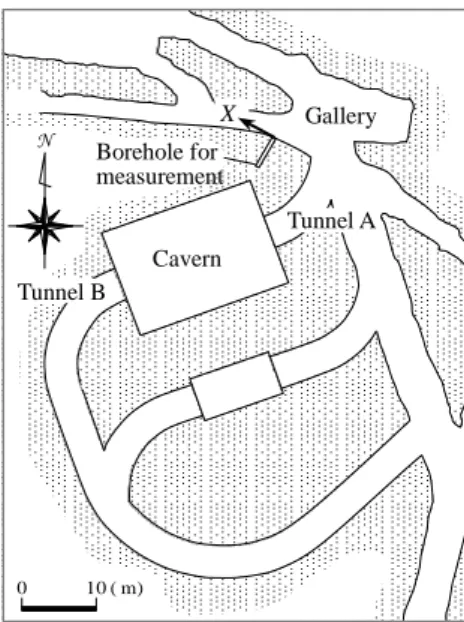
The plan view of the measurement site in Kamioka Mine is shown in Figure 14 (Obara et al. 2011b, 2012a, b). A cavern was excavated at a depth of 900m within gneiss. The Young’s modulus and Poisson’s ratio are 30GPa and 0.2, respectively. The dimension of the cavern is 15m by 21m and 15m in height. A borehole with a length of 5m for measurement of stress change was drilled horizontally from the gallery to the cavern before the start of its excavation.
The width of the rock between the gallery and the cavern is about 7m. The borehole for measurement was drilled in the wall. The four measuring points are located at depths of 1.0m, 1.8m, 4.0m and 4.5m, as shown in Figure 15. The measuring points are determined from the condition of the recovered core.
The excavation process is shown in Figure 16 in three dimensions. Firstly, the lower part of the cavern was excavated from access tunnel A. Then the upper part was excavated from access tunnel B. Finally, the middle part was excavated. The excavation method was blasting and its period was about six months for the whole of stages I to IX. The measurements were performed at nine stages before, during, and after excavation.
5.2 Measurement results
The results at a depth of 4.0m are shown as an example.
The measured and corrected displacements of the borehole wall at Stages V of the excavation are shown in Figure 17, assuming that the borehole radius is 37.85mm. The radius is not a real value but an expedient assumed one for calculating temporal stress. The solid line is approximation by the equation of the ellipse. The distributions of displacement in the measured results have a period of 2. However, applying both the non-linear least square method and non-linear programming for optimization to the measured results, the corrected data for eccentric positioning of the instrument changes to have a period of. The corrected data vary slightly, but represent a fairly good approximation. In Figure17(c), the cross-sectional shape in the plane perpendicular to the borehole axis is shown, adding 50 times
displacement to the radius. The shape is represented by an ellipse. The principal direction of the absolute stress state can be confirmed from this shape, although its value cannot be estimated from the CBDM.
Table2. Estimated temporal stress and stress change in the case that SY is changed from 3MPa to 5MPa.
Estimated temporal stress X Y XY
In the case of SY = 3MPa 3.52 6.32 -0.41 In the case of SY = 5MPa 3.45 8.03 -0.57
Stress change X Y XY
Applied stress change 0 2 0
Estimated stress change -0.07 1.71 -0.16
Figure 16. Measurement stage for the excavation of the cavern: access tunnel A is linked to (II) of lower part and tunnel B is to (V) of upper part.
Stage I: Before excavation
Stage II: Excavation of center of lower part Stage III: During excavation of lower part Stage IV: After excavation of lower part Stage V: Excavation of center of upper part Stage VI: After excavation of upper part Stage VII: During excavation of middle part Stage VIII: Just after excavation of middle part Stage IX: Three months after completion of excavation
Tunnel A side Tunnel B side
(V) (VI) (VI)
(VII)
(II)
(IV) (IV)
(VIII)
0 10 ( m)
N Borehole for measurement
Gallery
Cavern
Tunnel A
Tunnel B
X
Figure 14. Location of borehole for measurement and cavern in the plan view of measurement site in Kamioka Mine.
0cm 182cm 100cm
450cm 400cm
Figure 15. Core of borehole for measurement and measurement points.
-2 0 2 4 6 8 10 12 14
(Ⅰ) (Ⅲ) (Ⅴ) (Ⅶ) (Ⅸ)
X , MPa
Stage of excavation
-2 0 2 4 6 8 10 12 14
(Ⅰ) (Ⅲ) (Ⅴ) (Ⅶ) (Ⅸ)
Y , MPa
Stage of excavation
-10 -8 -6 -4 -2 0 2 4 6
(Ⅰ) (Ⅲ) (Ⅴ) (Ⅶ) (Ⅸ)
XY , MPa
Stage of excavation
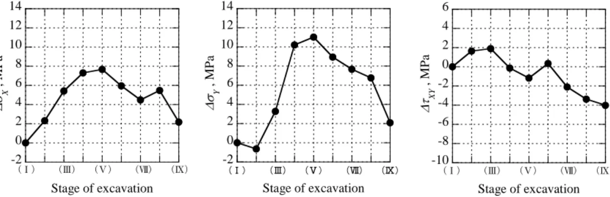
Figure 18. Changes of all components of stress in the X-Y coordinate system: X-axis is defined in the horizontal direction as shown in Figure 14 and Y-axis is defined vertically.
Figure 17. Measured and analyzed results: (a) measured data, (b) corrected data, (c) cross-sectional shape in the plane perpendicular to the borehole axis at Stage V; solid lines in (b) and (c) are approximations; deformation in (c) is described, adding 50 times displacement to radius.
-40 -20 0 20 40
-40 -20 0 20 40
Y , mm
X , mm -1
-0.5 0 0.5 1
-90 -45 0 45 90 135 180 225 270
Displacement, mm
, degree
-0.3 -0.2 -0.1 0 0.1
-90 -45 0 45 90 135 180 225 270
Displacement, mm
, degree
(a) (b) (c)
Figure 19. Distribution of stress change along borehole axis: (a)X, (b) Y, (c) XY, (d) vertical cross section.
-8 -4 0 4 8 12
0 1 2 3 4 5 6 7
X, MPa
Distance from gallery wall, m (IV)
(V) (VIII)
(IX)
-8 -4 0 4 8 12
0 1 2 3 4 5 6 7
Y, MPa
Distance from gallery wall, m (IV)
(V)
(VIII) (IX)
(II) (V) (VI)
(VIII) (IV)
(VI)
Gallery (IV)
15 m
22.5m Borehole for
measurement: 5m Cavern
8m 7m
3m
-8 -4 0 4 8 12
0 1 2 3 4 5 6 7
XY, MPa
Distance from gallery wall, m (V) (IV)
(VIII) (IX)
(a) (b)
(c) (d)
5.3 Change of stress distribution
The stress change at the depth of 4.0m during the excavation is shown in Figure 18. Since the initial stress state is not measured in this location, the stress change is calculated to subtract each component of the temporal stress at Stage I from that at any stage respectively. The vertical stress change Y is zero until stage II, but increases at stage III, then reaches the maximum value at stage V. After that, the stress decreases gradually with the progress of excavation.
The tendency of the horizontal stress change X is almost the same as that of Y. It is considered that the rock near the measuring point was damaged and became the loosened zone.
However, as the change of all stress components is continuous, it is also considered that that damage did not happen suddenly.
Finally, the distributions of stress change along the borehole axis at some stages are shown in Figure 19. The vertical cross-section along the borehole axis is in Figure 19 (d). The width of the pillar between the gallery and the cavern is 7.0m. In shear stress change XY of Figure 19 (c), the stress change is relatively small along the borehole axis during excavation. This means that there is not very much change in principal direction with elapsed time and geometry of cavern.
The vertical stress change Y in Figure 19 (b) is comparatively large. The stress change Y at a depth of 1.0m is small. As this point is near the gallery wall, the rock mass in this area is considered to be damaged. On the other hand, the stress change at a depth of 1.8m, 4.0m and 4.5m is large in early stages of the excavation. At a depth of 1.8m, the stress represents the maximum value at Stage IV, then it decreases to a half of the maximum value at Stage V. This value is maintained until Stage IX, which is completion of excavation. This means that the rock mass near a depth of 1.8m was not damaged. On the other hand, the stresses at depths of 4.0m and 4.5m also represent the maximum value at Stage IV, then they decreases gradually with the advance of the excavation. At Stage IX, the stresses decrease to the stress level lower than that before excavation. It is considered that the rock mass near depth of 4.0 - 4.5m was damaged due to excavation. These trends can be seen in horizontal stress change X shown in Figure 19(a). However, the state of the damaged zone is not clear. Therefore, that state should be confirmed by other methods such as numerical methods.
6. CONCLUSIONS
The Cross-sectional Borehole Deformation Method (CBDM) for measurement of rock stress change was introduced. Firstly, the principle of measurement was described, as well as the non-contact typed instrument with a laser displacement sensor. Secondly, the factors which affect measurement result were investigated theoretically, then it was shown that the eccentric position of the instrument is the most significant factor. A non-linear programming for optimization with the non-linear least square method was introduced in order to correct the eccentric position of the instrument. The applicability of it was shown based on the results in the laboratory experiment. Finally, the successful application to measure stress change under the excavation of a cavern was demonstrated. From the results, it was
concluded that the CBDM is available for measuring stress change.
REFERENCES
Berard, T. and Cornet, F.H., 2003. Evidence of thermally induced borehole elongation: a case study at Soultz, France, Int. J. Rock Mech. Min. Sci. & Geomech. Abstr., 40:
1121-1140.
Ibaragi,Y. and Fukushima, M., 1991. FORTRAM77 Saiteki-ka Programming, Iwanami Computer Science, Iwanami Shoten Publishers, pp.133-140.
Jaeger, J. C. and Cook, N. G. W., 1979. Fundamentals of Rock Mechanics, 3rd ed., Chapman & Hall, London, Chapter 10.
Kanagawa, T., Hibino, S., Ishida, T., Hayashi, M. and Kitahara, Y. 1986. In Situ Stress Measurements in the Japanese Islands, Int. J. Rock Mech. Min. Sci. & Geomech.
Abstr., 23: 29-39.
Kawabe, K., Sugimoto, F. and Imai, T., 2005. Development and Verification of Applicability of a Borehole Meter Using Laser Displacement Sensor, J. of MMIIJ, Vol. 121, No.8, pp.378-386.
Kiguchi, T. and Kuwahara Y., 2013. New Methods for Estimating Shallow Crustal Stress Orientation from Borehole Creep Deformation after Drilling, Proc of 6th Int.
Symp. on In-Situ Rock Stress, pp.1064-1074.
Kudo, K., Koyama, T. and Suzuki, Y., 1998. Application of Numerical Analysis to Design for Supporting Large-scale Underground Caverns, J. of Construction Management &
Eng., JSCE, 588, VI-38, pp.37-49.
Obara, Y., Matsuyama, T., Taniguchi, D. and Kang, S.S., 2004. Cross-Sectional Borehole Deformation Method (CBDM) for Rock Stress Measurement, Proc. of 3rd ARMS, 2, pp.1141-1146.
Obara, Y., Shin, T., Yoshinaga, T., Sugawara K. and Kang, S.S., 2010. Cross-Sectional Borehole Deformation Method (CBDM) for Measurement of Rock Stress Change, Proc. of 5th ISRS, CD.
Obara, Y., Shin, T., Yoshinaga, T., 2011a. Development of Cross-Sectional Borehole Deformation Method (CBDM) for Measurement of Rock Stress Change, J. of MMIJ, 127, pp.20-25, in Japanese.
Obara, Y., Fukushima, Y., Yoshinaga, T., Shin, T., Ujihara, M., Kimura, S., Yokoyama, T., 2011b. Measurement of Rock Stress Change by Cross-Sectional Borehole Deformation Method (CBDM), Proc. of ISRM 12th Int.
Cong. on Rock Mech., pp.1077-1080.
Obara, Y., Yoshinaga, T., Shin, T., Kataoka, M., Yokoyama T., 2012a. Applicability of Cross-Sectional Borehole Deformation Method (CBDM) to Measure Rock Stress Changes through Laboratory and In-Situ Experiments, J. of MMIJ, 128, pp.134-139, in Japanese.
Obara, Y., Kataoka, M., Yoshinaga, T., 2012b.
Cross-Sectional Borehole Deformation Method (CBDM) for Measurement of Rock Stress Change and its Application, Proc. of the 4th Traditional International Colloquium on Geomechanics and Geophysics, pp.13-15.
Taniguchi, D., Yoshinaga, T. and Obara, Y., 2003. Method of Rock Stress Measurement Based on Cross-Sectional Borehole Deformation Scanned by a Laser Displacement Sensor, Proc. of 3rd ARMS, pp.283-288.