Three types of location problems with the block norm

Three types of location problems with the block norm

著者 金 正道

year 1998‑03‑25

URL http://hdl.handle.net/2297/30583

Three t y p e s  o f  l o c a t i o n  problems with t h e  b l o c k  norm 

(ブロックノルムを用いた

3

タイプの配置問題)

金

.正 道

平成

1 0

年

1

月

¥ /  

博 士 論 文

Three types of l o c a t i o n  problems with the b l o c k  norm 

(プロックノルムを用いた

3

タイプの配置問題)

金沢大学大学院自然科学研究科 シ ス テ ム 科 学 専 攻 シ ス テ ム 基 礎 理 論 講 座 学 籍 番 号

94‑2  2  0  4 

氏 名 金 正 道

主 任 指 導 教 官 名 久 志 本 茂

Contents

1 Introduction ...

2 The block norm ...""...m...m...".."...

3 EtiEiciency ...

4 MSP with the block norm ...

5 MCP with the block norm ...

s.1 The determination ofE(Y) ...

s.2 The determination of QE(Y) ...

6 Application of MCP ...

7 Conclusions ...

1

3

7

11

20

20

22

25

30

1 Introduction

Given demand points on a plane, a problem to locate a new' facility on t,he plane is called a single facility location problem. The problem is usually formulated as a

minimization problem with an object,ive function involving distances between the facilit,y

and demand points.

On a plane, it is aAgsumed that, n<>-. P") distinct demand points yi (i R2, i = 1,2, • • • ,n and the distance is given by some norm II • ll. Let x E R2 be the location of the facilit.y

to be located, 'tvi > O be a weight for each yi and Y be the set of all demand points.

We consider t,hree ty. pes of objective functions:

(i)

n F(x) = 2w,lix -- yill•

i=1

(2)

G(x)=max{wdlx ---- yill : i =1,2,•••,'n}.

(3) H(x) = (Ilx - yi ll, Hx - y2H,•••, llx - y. ll)•

Problems to minimize objective functions F, G and H are known as, respectivel: , a min- isum Iocation problem(MSP), a minimax location problem(MMP) and a multicriteria location problem(MCP). If the facility to be located is public and not emergency, t,hen MSP and MCP can be used. If it is public and emergency, then MMP can be used. Let S.'vsp and S.'MMp be sets of all opt•imal solut•ions for MSP and MMP, respectively. MCP

is a problem to find an efficient or quasiefficient point. A point x E R2 is efficient if there

is no y E R2 such that lly --- y,II ff{ IIx -- y,II for all i and Ily -- yjII < llx- yjll for some ]'. An eflicient point x is alternately efllicient if there exists y #l x such that lly -- yAl =

llx -- yiil for all i. An efficient point x is strictly eflicient if x is not altemately efficient.

A point x E R2 is quasiefficient if there is no y E R2 such that IIy -- yill < llx- yAl for

all i. Let E(Y),AE(Y),SE(Y) and QE(Y) be sets of all efficient, altemately efficiellt,

strictly efficient and quasiefficient points, respect,ively. By these definitions, Y c SE(Y)

c E(Y) c QE(Y).

Various distances or norms are used in }ocation a,nalyses[2-8, 10, 11, 13-16, 19, 20,

22, .9.4, ,P.7, 27-321. For example, (', dist,ances(LP), t/he onp.infinity norm(OI), the A-

distance(AD) and the block norm(BL) are used in the above location problems as in

Table 1. The ei dist,ance is t,he rect,ilinear distance(RC) and tthe e2 distance is the

Euclidean distance(EC). The ei distance, the one-infinity. norm and the A-distance are

special cases of the block norm.

Ta,ble 1

References.

Distance

MSPMMPMCP

RC [5][6,8][2,32]

EC [5,19][6,8,10,11][27]

LP _OI [28][28][29] [5][6][27]

AD (13,14,16][22]Å~

BL [27,30][30][24,27,29]

Using the block norm, MSP and MMP are reduce(1 to linear programming prob- lems[30]. If the objective frmction G(x) for MMP is modified to incline slight,ly for

some direction, then the Exchange Algorit,hm in [4] to find an opt,imal solution can be applied to this problem. Its algorithm is an iterat,ive a}gorithm and generates a finite sequence of points converging to an optimal solution with O(n4) computational time.

For MCP under the block norm, algorithms to determine all efficient and quasiefficient point,s are given in [24], and t,hese algorithms require O(n2) and O(n) computational

time, respectively.

In this article, MSP, MMP and MCP with the block norm are con,gidered. First, eMcient points for MCP are characterized by using optimal solutions for MSP and MMP. Next, algorithms for MSP and MCP are considered. Fer MSP, the Edge Tracing Algorithm to find all optimal solutions is proposed. For MCP, two new algorithms to

find all eflicient and quasiefficient points are proposed. One is the Stairs Algorithm to find all efficient points. The other is the Wrapping Algorithm to find all quasiefficient points. It is shown that both of these algorithms are optimal in the sense of the order for

the computational time. Moreover, MCP is applied to the development of new products for the market of ready-made clothes.

In section 2, some properties of the block norm are given. In section 3, eMcient

points are characterized by using optimal solutions for MSP and MMP. In sect,ion 4,

t•he Edge Tracing Algorithm is proposed. In section 5, t,he Stairs Algorithm and the

Wrapping Algorithm are proposed. In section 6, MCP applied to the development of

new products for the market of ready-made clothes. Finally, some conclusions are given

in section 7.

2 Theblocknorm

In this section, some notations are prepared, the block norm is defined and it,s fundamental properties are given.

Let B c R2 be a bounded convex polyhedral set such that it is symmetric around

the origin and its interior contains the origin. Let ei,e2,•••,e2. be all extreme point•s

of B. For a E R2, a can be represented as a = llall2(cos a, sin a)

where ll • "2 is the Euclidean norm. An angle or is called an angle for a. For convenience of explanation, we set

aj• --- (a;,aS4), 2' =O,1,2,•••,2m+2

and Iet ori• be an angle for each aj•, where

{aj:]' ---= 1,2,•••,2m}= {ej:2' --'= 1,2,•••,27n}, O SII Ctl < Chf2 < ••• < CV2. < 2T, aj --- aj-2., 2' ----: 2m,2m+1,2m+2 and

orj ---- 2- + aj-2., 1' --"-= 2m, 2m + 1, 2m + 2.

Namely, a]•'s are ordered counterclockwise. N'ote that aj --- aj-. for ]' -> m. For x E R2, it is considered cones with a vertex at x generated by txAro adjacent vectors aj and a]•+i. Then we set

Qj (x) = x + e{aj, aj+i}, 1' --- O, 1, • • • , 2m

and

([?2m+j (x) = Qj (x), ]' '-:--- 1, 2, • • • , 2m - 2

where C{a,•,a,•+i} = {Aaj + JtLaj+i : A,xL }) O} (Figure 1). A cone Q(x) with a vertex

at x is type r if

i+r-1

([?(x)- U Qj(x) 2'=i

for some 2" (r == 1,2,•••,O-m). In particular, if Q(x) is type m then it is a half plane,

and if type 2m then it is R2. The opposite of a cone Q(x) is denoted by Q-(x), i.e.

Q"- (x) - 2x - Q(x),

and the set of all type r cones by R(x), i.e.

R(x) = {(?(x) c R2 : (?(x) is type r,r= l,2,•••,2m}.

a4

a2

al

Q3(x)

92(x)

Qi(x)

as

m=3

Q4(x) x

Qs(x)

q,(x)

Figure 1.

For each demand point yi and a2•, we set

Lij '-- {yi + oraj : or E R}.

It is an a2•-oriented line which passes through yi, For L,-j• 7C Liti, an int,ersection point of Li2- and Li,j•, is called an intersection point for the demand points set Y. Let I be the set of all intersection points for Y, i.e.

I == U (L,,- fi L,•jt).

i,i' ,1' 7Eji

A convex polyhedron S c R2 is called a region if all boundary lines of S are some of

Li,•'s, intS 7E Åë and (intS)nLi, == Åë for all Lij, where intS is the interior of S (Figure

2). Namely, any region S can be represented as

n

s = A Qj(i)(yi) i= 1

for some 1' (i)(1 .<-- 1'(i) .<. 2m). For any ar Åë Ui,j Li,•, let S(x) be a region whose interior

contains x. S(x) is called a region characterized by x, and is determined uniquel: by

(?j(i)(yi),i '--- 1,2, • • • ,n which contain x.

XXNX,Å~intersectionpoint

forY

s

Figure 2. al = O, a2

e

T/4, a3 = rt /2, a4 = 3T/4(m demand points

= 4)

Definition 1. Let B c R2 be a bounded eonvex poZyhedra

sy7Tt,metric arozL7?,d the ori,gin ana its interior contains the x E R2, lix", is defined as

Z set such th at it is

origin. The block norm of

(4) ^llxli --- inf{pt > O : x E tLB}.

From the above de

as follows[27,30].

finition

, B is an unit ball for th

e block norm.

llxll can be represented

(5) ^llxll

= mln { ^{2 1or m}

2'---1

m jl :x =2

J'---1

7jaj }

Therefore

tlons a]•r]

Ilxll can be regarded as the shortest pat•h from the origin to x using orienta-

= 1,2,•••,2m. From (4) and (5), we also have following lemmas.

Lemma 1. ^{For x =(vi}

^{1 iu 2}

⁾

^{E ([? j (o),}

(6) ^IIxll

:z• ' (al4+i - ai2. ) + z'2(a Ji

-- a3i•+i) a;• a34+i

-- a;•+ia]2

Proof. Consider the equation in 'rj• and 7'j•+i

x == rjaj + rj+laj+1•

From (4) and (5), llxli == r,- + r,•+i. Since ajr and aj•+i are linearly independent, i 2 1 i 2(aj2• +i x'i - a;• +i a:2, -aj2. cci + a; x•2).

(r]•, rj• +1) =

ajaj+1 - a]• +1aj•

Hence (6) is obtained.

Lemma 2. For a] == (xi, c2),y= (yi,y2) anaz=(z•i,z2) such that x E ([?j(y) z E Qm+,•(Y),

llx - zll = "x -yll + ll3y -zll•

Proof. Without loss of generality, we set y == (O,O). By Lemma 1, z"(a,2•+i -- a,2•) + a'2(a,i• - a}+i)

llxll = a; a?.+i - a}+iaj2'

zi(a2.+j•+i - aZ+j•) + 22(ae.+j - a;n+j+i) and

llzll --

-aj and x

h+j+ia%+j

- 22

)(aji. -- a;•+i)

we have

D

and

Since a,n+j =

llxll + 11zll

In the foliowing,

ain+2•aZ,+,•+1 - a - z E Qj (o),

(xi -- zi)(a]2•+i - a,j2•) + (x2 '-

a; a22• +i-a;• +iaJ2•

it is assumed that the block norm is given.

llx-zll

o

3 Efficiency

In this section, efficient points for MCP are characterized by using optimal solutions

for MSP and MMP.

In MCP, following propositions are given in [241.

Proposition 1. x Åë (?E(Y) of and only if R(x) contains at least one cone Q(x) such that it is tmpe m and Q(x)AY == Åë.

Proposition 2. Forx E ([?E(Y),

(i) x E (?E(Y)XE(Y) if and only if R(x) contains one cone (2(x) szech that i,t is type rrt -- 1 and (2(x) fiY=Åë and int(2-(x)nY i7E O.

(ii) x E AE(}"') if and only if R(x) contains one cone q(x) suclt that it ?is type m- 1

and (9(x) fiY == Åë and intQ-(x)nY == O.

(iii) x E SE(Y) if and only if R(x) does not contain any cone (?(x) such th,at it is

type m-1 and (2(x)nY = O•

From the t•heory of vector valued convex programming problems, the follow'ing the- orem is shown easily ( See Theorem 1 of Lowe et al.[21]) .

Theorem 1. x' E (?E(Y) if and only if there exists a vector w = (wi,w2,•••,wn) 2 o

siLch that w i7E o and x' is an optimal solutton for MSP with. weights wi,w2,• •• ,w..

Using the block norm, we have the follewing theorem which characterizes eMcient points for MCP by optimal solutions for MSP.

Theorem 2. x' E E(Y) if and only if there exists a uector w = (wi,w2,•'',wn) > O

siLch that x' is an optimal sohttion for MSP with weights iL]i,iv2,•'•,wn•

Proof. (<==) Assume x' Åë E(Y), then there exists y E R2 such that

lly - yi ll ff{l llx' - yi lls i = i, 2, • • • , 7?•,

and

lly- yjll < IIx' - yjli for some i

Therefore, in the objective function F for MSP, we have

n rt

F(y) = 2 willy - yill < 2 iL]illx' - yill = F(x')•

i==1 i.---1

This contradicts the optimality of x'.

(==>) Let, B' c R2 be a bounded convex pelyhedron whose interior contains x'. XAIe

set

P= {z = H(x') --- H(x) E R" : x E B'}

where ll is the objective functtion for ]VICP. Since x' E E(Y), we see t,hat therp is no

y E R2 such that

lly- yill f{{ IIx* - yill,i -=-• i,2,•••,n,

and

lly -- yjil < 11x' -- yjII for some i Therefore

pfi R". --- {o}

where R"

+ = {z E R't : z }lr o}. By the convexity of each llx -- yill, we have

(rcP) n R4 - {o}

where ,AC'P is a convex hull of P. Since (,ACP) n(intRZ) = Åë, there exists a separating hyperplane of KP and intRZ, i.e. t,here exist nonzero vector w E R't and b E R such

that

<w,zi> >.b>- <w,i2>, zi EitntRn., z2 E ICP

where <•,•> is the inner product. Now we see that w 2 O and b= O. Therefore <W, Zi> )0) <w, z2>, zi E R"+, z2 E ]<I P.

Let Si,S2,•••,Sq be all regions. Since each llx --- yill is linear in x on each region by

Lemma 1, H(Si fi B') c R", i --- 1,2,•••,q are bounded convex polyhedra. Since

9

P == H(x') -- U H(S, fi B'), i=1

rcP is a bounded convex polyhedron. Therefore we can choose w > o such that <zv,z2> S O, z2 E P.

From the definition of P

'

<w,H(x') - H(x)> .<.- o, x E B'.

Hence vtTe have

nn

2) wi llx* - yili S 2 wi ilx - yi ll, x E B"

i=1 i=1

where iv = (wi, iL,,2, • • • , zL7.). By the convexity of F, x' is an optimal solution for MSP

with such weights wi,w2,•••,'w.. M

For the optimal solut/ions set SXiMp of MMP, we have the following lemma.

Lemma 3. SMMp is a point or a line segment.

Proof. Let• t' be the optimal value for MMP. Since MMP can be rewritten as

min t

s.t. willx -- yill :f{l t, i --- 1,2,•••,n, S,*vMp can be represented as

n

SMM. = n{x E R2 : w,llx -- y,s{ s t*}.

i=1

Thus SMMp is (i) "a point" or (ii) "a line. segment" or (iii) "a bounded convex polyhedron

whose interior is not empty". We show there is not the case (iii). Assume that SMMp is a bounded convex polyhedron vvThose interior is not empty. For hi E intSXiMp,

wi ll ir' - yi II S G(2if), i ---- 1, 2, • • • ,n

and

wi,llirf - yi,ll = G(II!) for some i' where G is the objective function for MMP. Since yi, E (?j,(ZIi) for some i

and iE is an interior point of SMMp, for sufl}ciently small E > O,

y E (?;,(hi) n{x E R2 : Ilx- II!Il = 6} c intSMMp

satisfies the condition

(7) ivilllll7- yi ll S G(zz'), i --- 1, 2,•••,n.

By Lemma 2,

llllj' - yitll - Ilizj - iti'11 + "iif - yi•il.

Thus we have

wi,IIY- y,,li : 6iL?i, + wi,lilli - yi,il = 6w,, +G(IIi') > G(zli').

This contradicts (7). Therefore there is not t,he case (iii). O

It is shown easily that any optimal solut,ion for MMP is a quasieMcient point for MCP. Using the block norm, we have the following theorem vgThich characterizes efficient points for MCP by optimal solutions for MMP.

Theorem 3. Th,ere exists an optimaZ solution for MMP such that it is an efiicient pout for MCP,

Proof. For x* E SMMp, assume x' E (?E(Y)XE(Y). Since S,'vMp is a line segment by

Lemma3, for some xi,x2 E R2 such that• xi i7E x2, S,inip = Ixi,x2] = {(1---A)xi+Ax2 :

O -< N s{ 1}. Since x* gt E(Y), only one of following cases holds:

(a) For some uri c [m')xi],

ilx' - yi ll .< llx' --- zii ll, i = i, 2, • • • , `n

and

Ilx' - y,•Il < IIx' --- y,•II for some ]'.

(b) For some x" E [x',x2],

llx" --- yill -<-. "x' -yill, i• =: 1,2,•••,n

and

llx" - !ij ll < llx' - yJ- ll for some i

Without loss of generalit,y, it is assumed that the case (a) holds. For any x E Ixi,x21 and y Åë SMMi),

lly' yjil > IIa -- zijll for somei

Next, we show that there exists an efficient point Zi E [x',xi]. Assume that

(8) [x*,x,)AE(Y) =Åë

where ix',xi) = {(1 - A)x'+Axi:O s{ A < 1}. Note that each llx -- yHl is convex and piecewise linear on SXfMp in x. Thus, for sufficiently small E > O and some i,,

IIm' + A(xi --- x") - y-l is strictly decreasing in A E [O,6], Then we show that

(9) ]i'(1 -< i' -< n) s.t. Ilx*+A(xi -x')-y,,il is strictly decreasing in AE [O,1].

Assume that there is no i' in (9). If we set

Ai = max{pa E [O,1) : llx' + A(xi --- x') - sl,ll is strictly decreasing in A E [O, pa]}, i '---- 1,2,•••,n

and

Amax == max{Ai :i '-'-: 1,2,•••,n},

then x'+Amax(xi -- x') E [x',xi) is an efficient point. This contradicts the assumption

(8). Therefore (9) holds. If we set aT = xi, then "y - yjll > ll:I! - yjll for some ]' and

any y l Zi!. This means that t•here is no y E R2 such that

"y --- yi11 m< 11iiT- yill, i --- 1,2,•••,n,

and

lly - yjll < IIir' - yjll for some ]'.

By Theorem 2 and 3, an efficient point for MCP is a candidat,e of an optimal solution

for MSP and MMP.

4 MSP with the block norm

In this section, MSP with the block norm is considered. Properties of opt,imal

solutions for MSP are given and the Edge Tracing Algorithm to find all opt,imal solutions,

which requires O(n3) comput,ational time, is proposed.

Since the objective function F for MSP is a convex func.tio", MSP is a convex programming problem, Furthermore there exists an optimal solution for MSP. In the

optimal solutions set, SX,isp for MSP ai}d the set I of intersection points for the demand

points set Y, we have following theorems.

Theorem 4. The set I contains at least one opti,mal solution for MSP. Namely SX,.. AI l e.

Proof. For x' E SMspV, only one of following cases happens.

Case 1. For some region S, it is assumed that x' E i7'etS. Since F is constant on S, int,ersection points for Y, vvThich are vertices of a convex polygon S, are also optimal. Case 2. For some adjacent intersection point•s xi,x2 E I, it is assumed that x' == (1 -- A)xi +Ax2 for some A(0 < A < 1). Since the objective function F is constant

on [xbx2], xi and x2 are optimal. .

o

Theorem 5. Let Si and S2 be ad2'acent bounded regions, and let Si C SiVsp. Then sxf,. A(ints,) = o .

Proof. Assume t,hat ZIT E SX.fspn(intS2). For any x' E intSi, VF(x') = o. Namely Tl

(io) 2kt;i SV IIx'-yi ll =o.

i=1

In the following, we show that VF(ZE) l o which cont,radicts the assumption. For the purpose, some conditions are assumed without loss of generality. For convenience of explanation, we set

bj =aj+i -- aj, ]' -- O,1,2,•t•,2'nz,

and let 52• be an angle for each bj. Then, for each ,Bj, we set 6S• = 5,• - g and bS• = (cos 131.,sin /3;).

Note that bi.+j = -bS•. For x E i7!t([?j(y,), there exists k,• > O such that

(n) vllx-yi ll=kj bl•

by Lemma 1. Let xi and x2 be end points of a line segment Si n S2. It is assumed that

xi -- x2 has t•he same or]'entation of aj, (1 .< ]`' S m), that is, x2 -- xi has the same

orientation of a.+j•,. We partition the index set of demand points on a line patting

through xi a/nd x2 into two sets:

Ij, = {i :yi '--'- x2+orajt for some ty >O,1 f{{ i f{ 7't},

Im+jt = {z' : yi == xi+7a,.+jt for some 7>O,1 s{ i -< n}.

Note that Io•tUI.+,•, 7E O. Without loss of generality, it is assumed that Ij, il! Åë. For

i E I,v, since SinS2 C ([2.+j,-i(yi)fi(2?.+,v(yi), either (a) Si C (?.+j,(yD or (b)

Si C Qm+ji-i(yi) holds. It is suflicient to consider the case (a). It is assumed that the case (a) holds (Figure 3).

yi, iE Ji

Xl aj, .Å~

Si

X2

x a.+j"

Qm+i (Yi)

Figure 3.

Equation (10) can be rewritten aks

(i2) v7.F'(x')== 2 wiVIIx'-yAl+ 2 wiVlix'-yill=o•

4IjtUIm+j, iEI,tUIm+)i

For i Åë IjiUI,.+j,, since some type 1 cone (?j(yi) with a vertex at a demand point yi

contains Si and S2, VIIhi - yAl == llx' --- yAl. Therefore, from (12),

vF(zr') = 2 wiVllie'-yill+ 2 u;iV'ilzii'-yill iÅëIJ'UIm+J' iEIi,UIm+)t 2 ztJ,Vllzli'--y,ll- 2 iL;,Vllx*-y,II.

iEIjiUIm+j, iEI),UIm+j,

From (11), if i E J,•t then

Vllx' - yill = k.+jib'.+j,, VllZIi" -- yi" == km+j,-ib'.+j,-i

for some km+i,k.+j•tni > O, and ifiE I.+j, then

Vllx* -t y,ll = ki-,bl•i-,, V"hi - y,ll =: kj•bS"

for some kj•,-i, k2•i > O. Since

2 •u?iVIIx'---yiil E e{blv-i,bh+ji}X{o},

iE I), U Im+j'

2 wiVllziy-y,ll E e{bl•t,bh+ji-,}X{o}

iE Ij, U Irn+J'

and

(e{bl••-,, bh.,•} X {o}) fi<e{bSv , b;..,i-,} Å~ {o}) - Åë,

we have

VF(hi) = 2) wiVllhi - yi)l - 2 iviVllx' - fyill 7t< o•

iE Ij,UIm +j, iE Ij'UJrn +J'

Thus ZIY is not optimal. This contradicts the assumption. O

Next, an algorithm to find all optimal solutions for MSP is considered. By Theorem 2, efficient• set E(Y) contains SX4sp. However, for the simplicity of treatment, we use quasiefliicient set (2E(Y) instead of E(Y). Obviously, ([?E(Y) contains SMsp. It is the smallest convex polygon such that it includes all demand point,s and each boundary line

is a,•-oriented line for some J' by Proposition 1 (Figure 4). Note t,hat, each boundary line

of QE(Y) is a supporting line to the demand points g, et Y.

Yl

3

QE(y) Y4

Y5

2

Figure 4. (?E(Y), Y = {Yi, Y2,' ' ' , Ys}

a'i = O, Ctz2 == T/4, ai3 = 7r/2, cM4 = 37r/4(m = 4)

By Theorem 4, there exists an optimal solution x' E IA(9E(Y). So, in order to determine such an optimal solution, we propose the iterative method that traces onl:

intersection points for Y in (?E(Y). Let x(r) E I be a point after rt•h iterat•ion. NVe say ao• satisfies condit•ion (Q) for x(r) if there exist a demand point yi and 6 > e such that

yi = x(") +7aj for some ty E R

and

x(") +eaj E (?E(Y)•

We set

J == {2' :a,• sattisfies condition (Q) for x(r)}.

For the objective function F, we denote the right differential coefficient, of F at xo G R2

with respect to nonzero vector a E R2 as 0+F(xo;a), and set

(13) Ze (r) = i,i. i,i',n{0+ F(X(r)I a,)}.

If u(') ;l) O, then x(r) is optirnal by the convexity of F. B.y Theorem 5 and its proof, the optimal solutions set SMsp is "an intersection point for Y:' or "an aJ•-oriented ljne

seglnep,t for some ]', whose end points are adjacent intersection points for Y", or "a

reglon .

By Proposition 1, ([?E(Y) is characterized by L,j•'s where Lij• is an a,-oriented line

passmg through a demand point yi. For each aJ-, it is a. ssumed that n(2') lines are different among Li)-'s. We sort those lines according to y-interceptts if aj 7E T/O. and

x'-mtercepts if a]+ ---' z/2 in ascending order. For t•he simplicity of the notation, we write

the above sorted lines as '

q,es,•••, q, (j)

fer each a,• (Figure 5). Each line e'i(el',(j)) is called the bottom(top) line. Quasieffici'ent

set QE(Y) can be determined by at most 2m lines ejk' , ]' = 1,2,•••,2m;k = 1,n(]'), and

we arrange these lines as

(14) e,l,e2,,•••,eY-':eZ(,),eZt,'.,),•••,e.m(.):ek(,),eZ(,),•••,ezi,'-,):eg,el+i,•••,eln

LXg,9i?.i,g7'N6,g/,?,.f.Xqh.L.i?.P.S,,i,n.5,',l',,ft2e,8r.ia,8ig:.diF-81,8:e,g,vy.a8,9•E.(,Y,),go.Ei?l;'igT

For example, we consider the case n = m == 3 (Figure 5). We have el : eg,eg : eg : e?, e?

as arlanged lines. Nbte that n(1) = n(2) = n(3) == 3 and q = 2. A line el is the bottom

ai-oriented line. Lines e32,eg are the top a2-oriented line and the top a3-oriented line, respef'tively. A line ('3i is the top a4-oriented line. Lines e2i and ('3i are the bottoiiri as-orient,ed line and the bottom a6-oriented line, respectively.

'3

e.>

Yl

el

QE(y) ^Y3

cg

Y2

_eg

e? _eg

Fig

a'1 =

ure 5. e O.785, a2

: demand points

== T/2, a•3 = 2.678

Quasiefficient set QE(Y) can be represented by a system of inequalities for lines in

(14), i.e.

:': :g: g; tZ l. ke,, if a, g,

(?E(y)- (x•y): ft8 t,, ifaj i•

]' --- 1,2,•••,m

where bkj is y--intercept if aj 7C T/2 and x-intercept if cMj k-- T/2 for each eik. Note that

its system of inequalities may contain redundant inequalities. Now the procedure to remove such redundant inequalities is considered.

For t,he simplicity of the notation, let

e(1), e(2),•••,e(2m)

be lines in (14). Especially, we set e(2m + 1) == e(1) and e(2m + 2) = e(2).

The procedure to remove redundant inequalities for (?E(Y)

Step 1. Determine an intersection point of e(1) and e(2), and let zi be its intersection

point. Set 2' '-- 2.

Step 2. Det,ermine an intersection point, of e'(2') and e(1' + 1), and let zj• be its intersec-

t!on pomt.

Step 3. If zj '--- zj-i, then remove ('(7`).

Step 4. If 1' = 2m+1, then stop. Otherwise set j b-- j+1 and go t,o Step 2.

A system of inequalities for lines left after the above procedure does not contain any redundant inequality.

Now we give the Edge Tracing Algorithm to find all optimal solutions for MSP.

The Edge Tracing Algorithm

Step 1. Choose any demand point a,s an initial point x(O). (We choose a demand point with t,he largest weight.) Set r = O.

Step 2. Calculate ze(r).

Step 3. If ?L(r) > O, then stop. x(") is an optimal solution.

Step 4. If u(") = O, then stop. If ak whic.h satisfies u(r) = O is unique, then any point•

x E [x('), gcl.r)], where xfar) is an ak.-oriented adjacent intersection point for Y to

m(r), is optimal. Otherwise, for sufliciently. small E > O and ak(i),ak(2) which

satisfy u(r) = O, any point x E S(cc(r) + e(ak(i) + ak(2))) is opt•imal.

Step 5. If iL(r) < O, then choose any ak which satisfies ze(') = a+F(x(r);ak), and let x('+i) be an ak.-oriented adjacent intersection point for Y to x('). Set r == r + 1, and go to Step 2.

Choose x(O)

7' =O

Find iL(r)

r=r+1

_u(r)

N

)o ^{Y Stop}

Find x(T+i)

Flovvr chart of the Edge Tracing Algorithm.

The Edge Tracing Algorithm is convergent in finite iterations and requires O<n3) computational time, The number of intersection points for Y is finite and F(x(O)) >

F(x(!)) > ••• > F(x(")) from Step 5. Therefore The Edge Tracing Algoritdhm is con- vergent in finite iterations. The number of intersection points is O(n2). For a given x E R2, the complexity for calculating F(x) is O(n), so the complexity for determining

iL(r) in St,ep 2 is O(n). The complexity for det,ermining S(x(r) +s(ak(i) +ak(2))) in Step 4 is O(n), so the complexity of Step 4 is 0(n). The complexity for determining x('+i) is

O(1) when we have sorted lines, so the complexity of Step 5 is O(1), The complexity for

sorting n real numbers is O(n log n) [1], so the complexity for sortting lines is O(n logn).

Therefore the Edge Traci'ng Algorithm requires 0(n3) computational time.

If ah which satisfies 7L(') = 0+F(x("); ale) is determined in St,ep 5 of the Edge Tracing

Algorithm, we need to det,ermine x("+i) which is a•n ak-oriented adjacent intersection

point, for Y to a('). NText we consider the procedure to determine x("+i). For each a]•, we set

f,(.,,,) =( .-xtan Q] + ?y ll g; l /g,•

Then vf,(.,,) - ( Ei, ,t?n ai•i) li cr,,; l it•

It is assumed that an initial point x(O) = yi is given. Set r = O where r is a counter.

Let s(7';r) be an index of eZ` passing through x(r) (7' -"-t 1,2,•••,m). We concentrate on s(2';r), ]' -- 1,2,•••,m. It is assumed that ak in Step 5 is determined, and that k <- m without, loss of generality. For ]' 7E k (1 s{ j <-. m), set

tkj ---- <Vfj(x,y),ak>

and let zk.j• be an intersection point of

(ls) eg<k,.) and ej.'

(j,,)+s2gn(tk,)

where

,,g.(.) :( Å}l lff .x <> g:

for x f O. These intersection points zkj•:s are candidates for x('+i). Set (16) J(r) = (7 : llgc(') - zkv ll2 --- hÅ}kl}i}Iil,s.{Ilar(") - zkhll2}] •

Then x(r+i) is an intersection point of e,k (k,.) and E'].(,,,)+,ig.,(t,,), ]' E el(')• Set

(17)

t s`(]';r) if ]' ----; k,

s(1';r+1) = < s(]';r)+sign(tk,-) if ]' E ,J(r),

1 s(1' ; r) + O.5s z' gn (tkj ) otherwise.

If k > m, then reset k =k- rn and tkj '--' --<Vfj({r,y),ak>•

For all ]' such that b'(]';r+1) E N, x(r+i) is an int•ersection point of ('],'(j,.+,)'s, whp.re

N is .a set of natural numbers. For 2'

such that s(j;r) Åë N, x(') lies between ('jti.(,•,.)]

and el.(i,.)]+i where I•] is Gauss' symbol,

After the rth iteration, we have a point x(") with s(]•;`r), ]' --- 1,2,•••,m.

The above procedure is only the case of r = O. If r >- 1,then, in (15) and (17),

s(j'; 'r) + sign(tk.•) is replaced by

( [gEl•l•r,l;?i5] l•ig!,gy,.E:;.:- i,'•

and b'ign(tkj) in the third equation in (17) is replaced by s'ign(tkj)([s(]'.; r)l -- [s(1':r) -- O.51).

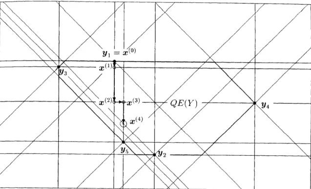
Next, vLre consider the following example prob}en} of a single facility minisum location

problem

5

.Illlli'Iii2 F(X)• -F (x) = l. III., Iix - yi ll

where

ai = (1,0), a2 = (cos 7r/4,sin 7r/4), a3 = (O, 1), a4 = (cos37T/4,sin 3T/4),

y, = (63, 97),y, = (102,7),y, =: (10, 90), y, = (197, 57), y, = (73, 20).

In this case, m=4, 'n '-- 5 and 'wi =: 'w2 == w3 = w4 = zvs =1. We set x(O) = yi as an

initial point, and appl: the Edge Tracing Algorithm to this probleizri.

1. (Step 1) The initial point is x(O) == (63,97) with

s(1;O) ----: 5,s(2;O) = 4,s(3;O) = 2,s(4;O) =4.

Go to Step 2.

2. (Step 2) We have zL(O) = 0+F(x(O);a7) == --1.828 < O. Go to Step 5.

3. (Step 5) We have k = 7, so x(i) is an a7-oriented adjacent intersection point for Y to x(O). Go to Step 2.

4. (Step 2) We have x(i) == (63,90) vv'ith

s(1; 1) == s(1; O) -1 =4 , s(2;1) = s(2;O) -- O.5 == 3.5 , s(3; 1) == s(3; O) =2 ,

b•(41 1) = s(41 O) -O.5 =3.5 .

Continuing the above procedure, we have x(2) = (63,57),x(3) = (73,57),x(`) = (73,36),

and zL(4) > O. The optimal solut,ion is x(4) = (73, 36), and the optimal value is F(x(`)) = 340.22 (Figure 6).

Yl=X

^(o)

x(1)

3x(2)

x(3)

x(4)

qE(Y) Y4

Y5

2

Figure 6. 0 :

the o ptimal solution, e :

demand points

5 MCP with the block norm

In this section, MCP with the block nonn is considered. Two algorithms to deter- mine E(Y) and QE(Y) are proposed. Furthermore it is shown that these algorithms are optimal in the sense of the order for the computational time.

Without loss of generality, it is assumed that

O'j

i=- 7r /2 for all j. If

O'j =

7r /2 for some j, then rotate a plane counterclockwise for sufficiently srnall

E

>

0

and reset

O'j

=

^O'j

+

^E

for all j.

5.1 The determination of E(Y)

In this subsection, The Stairs Algorithnl to determine E(Y') is proposed. For each L

_{ij )}

if Lij = £{, then

we

set s(i,j) = k.

For each

e{, if

Yi is a den1a.,nd point with

maxilnulIl(minimum) x-coordinate among demand points located on £1, then we set (k,j)max = i((k,j)rnin == i). In the following algorithm, we set

p(e) = { 1 if 0 <

O'e

< 7r/2 or 37[/2 <

eYe

< 57r/2, n( c) if 7r /2 <

O'c

< 37r /2 or 57r /2 <

O'c

< 37r for c = 2,3,···, 2m + ^1,

q(c) = {+_11 if 0 ~

^O:c

^< 7r/2 or 37r/2 <

O'e

< 27r, if

7f

/2 ^<

^O'c

^{< 37r /2}

for

c

= 1,2, ... ,2m, and

( ) == { ^rnax

o

c .

mIn

for c = 1,2, ... ,2m.

The Stairs Algorithlll

if 0

~ etc

< 7r /2 or 37r /2 <

etc

< 27r, if 7r /2 ^<

^O'c

^{< 37r} /2

Step o. ^Determine ft, 8(i,j), (k,j)maxl (k,j)min, 1 ~ i ~

n,

1 ::; j ::;

2m,1 ::; k ::; n(j).

Step 1. If 0 ::;

^0'1

< 7r /2, then set

z*

=

Y(1,l)min' r

== (1,1 )max and d = 1. Otherwise set

z*

==

Y(n(l),l)max' r

==

(n(l),

1 )min and

d

==

n(l).

Store the route from

z*

to Yr. Set z = Yr and

c

= ^1.

Step 2. If

8(1', C

+ 1)

=

p(e + 1), then set d == p(e + 1), c == c + 1 and go to Step 2.

Step 3. If {J5(c + 1) - 8(1',

^C

+ l)}{s((d + q(c), c)o(e), c + 1) - 8(r, c + I)} 2: 0, then set z' =

Y(d+"q(c),c)<>(c)

and go to Step 4. Otherwise set d = ^d + 71( c) and go to Step 3.

Step 4. Let z" be an intersection point of t~t~c+l) and

fd+q(c).

Store the routes from z to z" and from z" to z', i.e. z

^---+

z"

^---t

z'. If z' == z*, then stop. Otherwise set

z == z'(==

Y(d+q(c),c)O(C))' r

= (d + q(c), c)o(c) , d == d + ^q(c)

and go to Step 2.

Let z'(z) be the demand point with minimum (maximum) x-coordinate among demand points located on the bottom ai-oriented line.

c= 1

Are there any demand points on Q.(z)X{z} ?

c----c+1

NT

Y

Let z' be the demand point on (2.(z)N{z} such

that, from z to the point, it has the farthest

a,-oriented subroute among demand points having the shortest a.+i-oriented subroute.

Store the shortest route from z to z'

a.+i first and then in a..

, gomg m

zt ==

N z=

z* Y

Zl

Stop

Flow chart, of the Stairs Algorithm when eq < T/2.

The stored route lines determine the boundary of E(Y). If there exists a region S

such that its boundary is a part, of the boundary of E(Y) and, for its interior point x,

Y C (?j,(x)UQ.+jt(x) for some i, then S : (2?j,(xi) fi (?.+j,(x2) where xi and x2 are

vertices of S such t,hat xi E (?.+j,(x) and x2 E (1?jt(x). Any point in SN{xi,x2} is an

altemately efficient point, and xi and x2 are strictly, efficient point•s (Figure 7).

Step O requires O(n logn) computational time[1]. In iterations from Step 2 to Step 4, c changes from 1 to P.m at most, and for each c, d changes from 1 to n at most.

Therefore this algorithm requires O(nlogn) computational time. Thus we have the following lemma.

Lemma 4. The Stairs AlgorithTn regzeires O(nlogn) computationaZ time.

Lemma 5. Any aZgorithm u7hich constrzects E(Y) reguires at Zeast O(nlogn) computational time.

Proof. Given n distinct numbers yi,y2,•••,y., it, is known that the minimum number of comparisons needed to rank the numbers is 0(nlog77.)[1]. We set yi ---- (yi,yi), i ---: 1,2,•••,n as demand points and consider the problem of determining E(Y). It is

assumed that aj 7E T/4 for all 1' and ai < 7r/4. For some ]" S m, Y C ([?jt(o) U (?.+,•,(o).

Let ((1]],[[2]],•••,(In]] be a permutation of 1,2,•••,n such that y[[i]] < y[[,+i]], i ---

1,2,•••,n-1. We set

E,'- =: (?j,(3y[[q]) fi ([?m+j,(y[[i.i]]), i = 1,2,•••,n -- 1

where y[[i]] = (y[[i]],y[[i]]) for each i. By the Stairs Algorithm, we see that

rt-1

E(Y) == U E;• . i=1

Any other algorithm to determine E(Y) would also need to specify each E,'• , which is completely determined by the numbers y[[i]] and y[[i+i]]. Hence it must be able to sort the numbers yi,y2,•••,y.. Therefore it requires at least O(nlog n) computational time.

a By Lemma4 and 5, w'e have the following theorem.

Theorem 6. The Stairs AlgorithTn, is optimal in the sense of the order.

5.2 TheDeterminationof9E(Y)

In this subsection, The Wi'apping Algorithm to determine (?E(Y) is proposed. For

each a,, let ej...(4 i.) be the line with maximum(minimum) y-int,ercept, among e]k' 's.

The Wrapping Algorithm

Step O. Determine e'.' ..,ei.'

i.,1 S j' <- 2m+2-

Step 1. If O s{ ai < 7r/2, then set e == ei:,i., otherwise set e = eeh... If O < cv2 < 7r/2, then set e' == eki., otherwise set e' = e2,.,.•

Let z be an intersection point of C' and e'. Set z* = z, e= e' and c =2.

Step 2. If O < cv,+i < T/2 or 3T/2 < (y,+i < 5z/2, then set e' = eC,,t/,1, otherwise set

et == ecfit.i..

Step 3. Let z' be an intersection point of e and e', and store the route from z to i'. If

z' : z', then stop, otherwise set

z == zt,e= et,c=c+1 and go to Step 2.

The stored route line.s determine the boundary of (?E(Y)(Figure 7).

Step O requires O(n.) computational time[25]. The number of iterations from Step 2 to Step 3 is 2m at most. Therefore this algorithm requires O(n) computational time.

Thus we have the following lemma.

Lemma 6. The Wrapping aZgorithm reqiLires O(n) comlnLtationaZ ti,me.

Lemma 7. Any aZgorithm which constructs (?E(Y) reqnires at least O(n)

computational ti,me.

Proof. Given n distinct numbers yi,y2,•••,y., it is known that the minimum number

of comparisons needed to find the maximum(minimum) number is O(n)I25]. We set yi = (yi,yD,i'--- 1,2,•••,n as demand points and consider the problem of determining

(?E(Y). It is assumed that Qi ff{ T/4. For some i S m, Y C (?j,(o)U([?m+j,(o)•

We set ymax = max{yi , y2, • • • , yn} and y.i. = min{yi , y2, • • • , y. }. By the Wr apping

Algorithm, we see that

QE(Y) = Qjs(y.i.)n([2m+j'(Ymax)

where y... = (ym..,ym..) and y.i. = (ymin,ymin). QE(Y) is completely determined by the numbers y... and y.i.. Hence any other algorithm to determine QE(Y) must be

able to find the numbers y... and y.i.. Therefore it requires at least O(n) computational

By Lemma6 and 7, we have the following theorem.

Theorem 7. The Wrappt,ng Aggorithm is optimaZ in the sense of the order.

Unit ball

SE(Y) AE(Y)

e

QE(y)

e

Figure 7. e:

demand points

6 Application of MCP

In this section, the development of new products for the rr}arket of ready-made clothes is considered an application of MCP,

A multivariate data which consists of individuals each of which has scores is con- sidered. First], tjhe data is analyzed by principal components analysis, and only t,wo principal components case is considered. Next, MCP using block norm for scores of principal components is considered. The block norm is defined to make up for t,he lost information due to principal components analysis, in a sense.

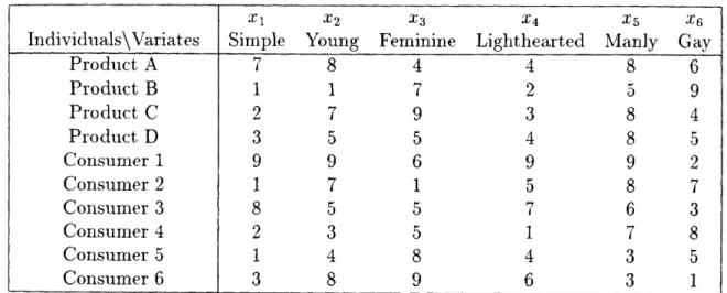
Consider the market of ready-rnade clothes. It is assumed that manufactured prod- ucts are characterized by some variates. Some enterprise wants to develop new products and there are candidates for new products A,B,C,D(Table 2). Are there any products better than these nevLr products? Then, six consumers are gathered information by

questionnaires for tastJe of products. In this case, characters of products and tastes of

consumers are measured in a common scale for common variates. Table 2 shews the

result.

Table 2. Characters o

f products and the result of questionnaires for taste.

Xl X2 ^Z'3 X4 X5 M6

IndividualsXVariat,es

Simple Young ^Feminine Lighthearted Manly Gay

ProductA

^{7 8 4 4 8}

6

ProductB

^{1 1 7 2 5 9}

ProductC

^{2 7 9 3 8} 4

ProductD

^{3 5 5} 4 8 5

Consumer1

^{9 9 6 9 9 2}

Consumer2

^{1 7 1 5 8} 7

Consumer3

^{8 5 5 7 6 3}

Consumer4

^{2 3 5 1 7 8}

Consumer5

^{1 4 8 4 3 5}

Consumer6

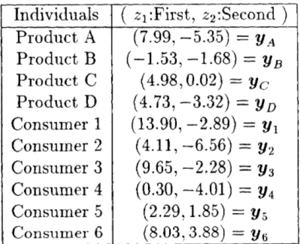
^{3 8 9 6 3 1}

For this data, Table 3

-e

varlance matrlx.

shows

^{the result}

of principal components

analysis

t from the co-

Table 3. Scores of principal component•s.

Individuals Product A Product B Product C Product D Consumer 1 Consumer 2 Consumer 3 Consumer 4 Consumer 5 Consumer 6

( zi:First, 22:Second ) (7.99, --5.35) = YA

(.-1.53, -1.68) = YB (4.98,O.02) = yc

(4.73, -3.32) = YD

(13.90, --2.89) = Yi (4.11, --6.56) = yr2

(9.65,-2.28) = Y3 (O.30, -4.01) = y,

(2.29, 1.85) = Ys (s.03,3.88) == Y6

Points yi , y2, • • • , y6 are dem and points in MCP, i.e. Y == {yi, y2, • • • , y6 }. A dem and

point yi represents a tast,e of consumer i and yA,yB,yc,yD represent, respect,ively, products A,B,C,D (Figure 9). Cumulative rate of contribution up to second component

is O.80. Table 4 shows correlation coefl}cient for each x,• and 2•k.

Table 4. Correlation coefficients.

Xl

O.86--O,21 ZlZ2

C2

O.83-O.03

X3

-O.04O.91

.T4

O.90O.08

X5

O.32-O.77

X6 --

O,82-O.53

Form this result, it can be regarded that zi means design and z2 means appeal to the male and female.

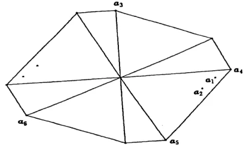
Next, an unit ball B which defines the block norm is determined. Table 5 shows

regression coefficient of zk on xJ• for each xj and zk.

Table 5. Regression coefficients.

(Zl,l2)

Xl

(1.28,-O.22)==ai

X2

(1.so,--o.o3)==a2

X3

(-O.07,1,18):a3

X4

(1.75,O.11)=a4

X5

(o.68,-1.l4)=as

X•6

(---1.45,-O.66)=a6

Then we set B == rc{Å}ai,Å}a2,••-,Å}a6}(Figure 8), Let m E R2 be a point which

represents a product. The distance between x and y,, llx -- yiU, is a degree of difference

between products x and taste yi measured by only vectors aj such that they influence principal components much. The block norm defined in this way can be regarded to make up for the lost information by principal components analysis.

a3

.

a4

s e

al

ai

k

as

Figure 8.

Unit ball B.

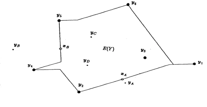
Next, MCP with the block norm defined as the above. In this section, efficient points

for MCP are considered. Figure 9 shows the result of MCP. If a product x Åë E(Y), then

it means that there is another product y E E(Y) better than x. Perhaps consumers

might buy products near their tastes. So, an efficient product y is more salable than a

product x which is not efficient. Therefore efficient set E(Y) can be regarded as a set

of salable products. Candidates for new products which are not efficient are modified

to be eMcient and minimize the cost to modify.

Y6 Y5

e

YB

Y4

2B

Y2

YD

e

yc

.

f

E(Y)

2A e YA

Y3 '

e Yl

Figure 9.

Eflicient set E(Y).

From the above result, products C and D are efficient but products A and B are not efficient. Hence products A and B should be modified. Here, it is assumed that the cost to modify a product y E R2 to x E R2 is E =: i("x - yll), where E is strictly increasing in llx -- yli. If a product yA is modified, then modified product xA E E(Y) is determined to minimize the cost to modify. It is similar for a product yB. By the

translation, without loss of generaJity, we set yA = o. Generally, for Y in section 1 and

the block norm in section 2, the problem is as follows;

(18)

min E(lixil)

s.t. xEE(Y).

Since e is strictly increasing in llxll, the problem (18) is equivalent to the problern

(19)

min Ilxil

sS. xEE(Y).

Since E(Y) is bounded closed set, there exists the optimal solution of the problem (19).

Theorem 8. Let x' be an optimal solution for the problem (19). If o Åë E(Y), then

x' Åë intE(Y).

Proof.

Assume that x* E intE(Y).

Then, for sufliciently small 6 > O,

(20)

{Y E R2 , lly-x'll SI E} C E(Y).

For some 1",o E (?

^j,(x').

Consider

(21) ^{II! E ([?}

,,(x*)Aq

^."7't

(o) A{y E R2 :

lly - Åë'H : 6}.

Then zrf E E(Y) by (20), o E ([?j,(iiT)

Ilx*ll = llx' -.

a•nd x' hiIl + Ii -

E (97•,(:i) by (21). By Lemma 2,

hill = s + 1keil > liasll•

This contradicts the assumption.

By the Stairs Algorithm, E(Y) is given by an sequence of points whic polygonal boundary of E(Y). Hence if o Åë E(Y), then the problem (19) the following problem by. Theorem 8.

For xi,x2 E R2 such that xi 7E x2 and o Åë [xi,x2],

h represent is reduced to

0

the

(22)

min

s,t.

llxll

x E [Xi,X2].

Next, an algorithm to solve the problem (22) is considered. For each a,•, let e,• be an

aj-oriented line passing through the origin, Let xi, x2 and intersection points of ej's and

[xi,x2) be pi,p2,•••,p,t from xi to x2. We set h(A) = ll(1 --- A)xi +Ax2Il,OS A -< 1

and pi "--- (1 - Ai)xi +Aix2,i= 1,2, •••,g' - 1. The right differential coefficient of h at Ai is denoted by 0+h(Ai). Note that "xll is linear on each tpi,pi+i] and piecewise linear

and convex on [xi,x2] by Lemma 1. In this case, the problem (22) can be solved by the following algorithm.

The Algorithm Step

Step

1. Set r=1 and x' =p,.

2. If 0+h(A.) > O, then stop, x' = p. is optimal.

X E [P.,P.+i] is optimal. If r = g' -1, then stop.

set r == r+1 and go to Step 2.

If 0+h(A,) = O, then stop. Any pq, = x2 is optimal. Otherwise,

From the above algorithm, we have xA == (7.72 which miniinize the cost to modify (Figure 9).

, -4.90) and xB =

^{(2.49, --} 1.44) as points

7 Conclusions

We considered a minisum location problem(MSP), a minimax location prob- lem(MMP) and a multicriteria location problem(MCP) with the block norm. For these problems, relations between optimal solutions were investigated, and algorithms to solve them were proposed. Moreover an application of MCP was considered.

First, we proved that the following relations: (i) An: eflicient point for MCP is an

optimal solution for MSP with some positive weights, and any optimal solution for MSP

is an eflicient point for MCP (Theorem 2). (ii) There exists at least one optimal solution

for MMP such that it is eflicient for MCP (Theorem 3).

Next, for MSP, it was shown that at least one optimal solution was an intersection point for Y and that any optimal solution was quasiefficient (Theorem 2 and 4). A set of all optimal solutions is an intersection point for Y or a line segment or a region by

Theorem 2 and 5. Based on these results, we proposed the Edge Tracing A}gorithm with

O(n3) computational time to determine all optimal solut/ions. It is an iterat•ive algorithm

using the descent method, and generates a finite sequence of int/ersection points for Y converging to an optimal solution. Sorting Lij's pla.yed an important role to generat•e that sequence efficiently. We may need many iterations if the initial point is not nea,r to an optimal solution and there are a lot of demand points near the optimal solution.

In this sense, we need further research on the choice of an initial point.

Finally, for MCP, we proposed the Stairs Algorithm to determine E(Y) and the Wrapping Algorithm to determine QE(Y). The Stairs Algorithm requires O(nlogn)

computational time due to sort Lij's, and it is optimal in the sense of the order for the

computational time (Theorem 6). The Wrapping Algorithm requires O(n) computa-

t•ional time, and it is also optimal (Theorem 7). Furthermore MCP was applied to the

development of new products for the market of ready-made clothes. In addition to this

application, it seems that there are many ot,her applicat,ions of location problems.

Acknowledgments

The author gratefully thanks Professor Shigeru Kushimoto of Kanazawa University for his worthy suggestions and warm encouragement.

The author is also very grateful to Associate Professor Setsuko Sakai of Fukui Uni- versit,y and Professor Takashi Maeda of Kanazawa University for their suggestiye and helpful comments.

Without their kind and significant guidance, this work could not have been per-

formed. The author would like to express his heartfelt thanks to many people concerned

with this research for t,heir warmhearted encouragement.

References

[1] A. V. Aho, J. E. Hopcroft and J. D. Ullman, The design and analysis of computer algorithms, Addison-Wesley, Reading, MA (1974).

[2] L. G. Chalmet, R. L. Francis and A. Kolen, Finding efi7cient solutions for rectiZinear distance Zocation problems efficiently, Eur. J. Oper. Res., 6 (1981), 117-124.

[3] Z. Drezner, 0n minimax optimization problems, Math. Prog., 22 (1982), 227-230.

[4] Z. Drezner, On the complexity of the exchange algorithm for minima,x optimization problems, Math. Prog., 38 (1987), 219-222.

[5] Z. Drezner and A. J. Goldman, 0n the set of optimal points to the Weberproblem,

Trans. Sci., 25 (1991), 3-8.

[6] Z. Drezner and G. O. NVesolowsky, Single facility ep-distance minimax location, SIAM J. Alg. Disc. Meth., 1 (1980), 315-321.

[7] Z. Drezner and G. O. Wesolowsky, The asymmetric distance location problem, Trans. Sci., 23 (1989), 201-207.

[8] J. Elzinga and D. W. Hearn, Geometrical solutions for some minimax location problems, Trans. Sci., 6 (1972), 379-394.

[9] A. M. Geoffrion, Proper efiiciency and the theory of vector maximization, J. Math.

Anal. Appl., 22 (1968), 618-630.

[10] D. W. Hearn and J. Vijay, Efiicient algorithms for the (weighted? minimum circZe problem, Oper. Res., 30 (1982), 777-795.

[11] S. K. Jacobsen, An algorithm for the minimax Weberproblem, Eur. J. Oper. Res., 6 (1981), 144-148.

[12] M. Kon, Efiicient solutions for multicriteria location problems under the block norm,

Math, Japonica, 47 (1998), to appear.

[13] M. Kon and S. Kushimoto, A single facility locationproblem with respect to minisum criterion(in Japanese), RIMS Kokyuroku 864 (1994), 47-55.

[14] M. Kon and S. Kushimoto, A single focility locationproblem with respect to minisum criterion IL RIMS Kokyuroku 899 (1995), 142-149.

[15] ]VI. Kon and S. Kushimoto, On location proble7rbs ?mder the asymmetric rectilinear distance(in Japanese), RIMS Kokyuroku 981 (1997), 85-88.

[16] M. Kon and S. Kushimoto, A singZe faeility location problem u,nder the A-distance,

Journal of the Operations Research Soc. of Japan, 40 (1997), 10-20.

[17] H. Konno and H. Yamashit•a, Nonlinear proy(ramm,ing(in Japanese), Nikkagiren, Japan <1978).

(18] S. Kushimoto, The foundations for the optimiiation(in Japanese), Morikita Syup- pan, Japan (1979).

[19] H. W. Kuhn, A note on Fermat'b' problem, Math. Prog., 4 (1973), 98-107.

[20] R. F. Love, J. G. Morris and G. O. Wesolowsky, Facilities location: models &

methods, North-Holland (1988).

I21] T, J. Lowe, J. -F. Thisse, J. E. Ward and R. E. Wendell, On ej6Ecient sokttions to multiple ob2'ective mathematical programs, Manage. Sci., 30 (1984), 1346-1349.

(.P,2] T. Matsutomi and H. Ishii, Eacility location problem 2llith restricted orientati,ens(in

Japanese), RIMS Kokyuroku 798 (1992), 129-139.

[23] T. Okuno, MuZtivariate Analysis II(in Japanese), Nikkagiren, Japan (1976).

[24] B. Pelegrin and F. R. Fernandez, Determination of ejCiEcient points irb miLltiple-

objective location problem,s, ]N'av. Res. Logist. q., 35 (1988), 697-705.

[25] I. Pohl, A sorting problem and its compZexity, C. ACM, 15 (1972), 462-464.

[26] R. T. Rockafellar, Convex analysis, Princeton University Press, Princeton, N. J.

(1970).

[O.7] J. -F. Thisse, J. E. Ward and R. E. Wendell, Some properties of location probZems with block and roitnd riorms, Oper. Res., 32 (1984), 1309-1327.

[28] J. E. Ward and R. E. Wendell, A new norTrb for measuring distance which yieZds linear Zocatton problems, Oper. Res., 28 (1980), 836-844.

[29] J. E. Ward and R. E. Wendell, Characterizing ejff. icient points in location problems

under the one-infinity norm, in, J. -F. Thisse and H. G. Zoller, Eds., Locational analys'is ofpublic facilities, North Holland , Amst,erdam (1983), 413-429.

[30] J. E. Ward and R. E. Wendell, Using block norms for gocation modeling, Oper. Res., 33 (1985), 1074-1090.

[311 R. E. Wendell and A. P. Hurter, Jr., Location theory, dom,inance, aTt,d convexity, Oper. Res., 21 (1973), 314-320.

[39-] R. E. VV'endell, A. P. Hurter, Jr. and T. J. Lowe, E2Slicient points in location prob-

lems, AIIE Trans., 9 (1977), 238-246.

[33] P. Widmayer, Y. F. VV'u and C. K Wong, On some distance problems in jfixed

orientations, SIAM J. Comput., 16 (1987), 728-746.