1Introduction Classificationofcapillaryimagesbasedontheaveragecurvatureestimation

Classification of capillary images based on the average curvature estimation

C HUONG Ngoc Duy Hung ¹ , Kazuaki N AKANE ² , Takahiro I TO ³ , Itsuko H ASHIMOTO ^1,4

1 Graduate School of Natural Science and Technology, Kanazawa University, Kanazawa 920-1192, Japan

E-mail: [email protected]

2 Graduate School of Medicine, Osaka University, Suita 565-0871, Japan

3 Department of Computational Science School of Mathematics and Physics, Kanazawa University, Kanazawa 920-1192, Japan

4 Osaka City University Advanced Mathematical Institute, Osaka 558-8585, Japan

(Received December 26, 2012 and accepted in revised form February 12, 2013)

Abstract It is known that, the state of the capillaries represents the health condition.

Recently, a device has been developed which can take the image of the capillaries at the base of the nail of the middle finger. If the state of the capillaries can be quantified mathematically, we can use it as an indicator of health. In this report, a level set method is developed to extract the outline of the capillary effectively. We have applied this method to two distinctive types of capillary, and calculated the value of average curvature. The results coincide with the diagnosis of the medical doctor.

Key words: image processing method, capillaries, average curvature

1 Introduction

Capillaries send fresh blood to all the corners of a human body. If the capillaries are functioning properly, metabolism is carried out smoothly, and it is possible to maintain a healthy condition. The state of the capillaries is often changed by mental stress and irregular life and eating habits. These factors disturb the balance of autonomic nerves and cause abnormal state of capillaries. According to the theory of medical doctor S.

Ogawa ([7]), the information on the state of capillaries in the whole body is collected on

capillaries in the left third finger ([3]). From such a medical background, in recent years,

the medical examination by investigating the capillary of a fingertip is performed in some

medical institutions.

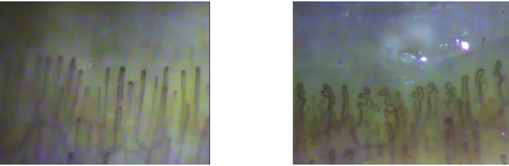
Figure 1: Example of images of capillaries, (Left) a normal state, (Right) an abnormal state, the capillaries are bent and the flow seems to be not smooth. The images are taken by a special device ([3]).

We can see different states of capillaries in Figure 1. From the diagnosis point of view, a healthy person has capillaries with the shape of straight line like in Figure 1 (Left). On the other hand, capillaries of an unhealthy person become wiggling like in Figure 1 (Right).

The purpose of this paper is to establish a method of extracting the outline of a cap- illary from digital images, and to give an index which expresses its state. Therefore, the index should be the value related to the curvature of the outline of a capillary. Generally, images contain noise and various artifacts. We should eliminate them and define an index which coincides with the medical diagnose.

Approximation method by solving the heat equation is often used to this kind prob- lems. Let Ω be a domain in R

on which the image is drawn. The function u(t,x) expresses a monochrome or a certain color shade. Because we treat digital images, the value of u is between 0 and 255. Here, by normalization, we suppose 0 ≤ u ≤ 1, where u(t, x) = 0 implies the color is white, while u(t, x) = 1 means x is black.

The heat equation approach considers the initial value problem with Neumann bound- ary condition:

 

 



 

 

∂ u

∂ t = ∆ u, in (0, ∞ ) × Ω , u(0, x) = u

(x), in Ω,

∂ u

∂ n = 0, in (0,T ) × ∂Ω .

(1.1)

If Ω = R

, it is known that the solution of (1.1) is written as u(t, x) = (G

∗ u

)(x)

=

∫

R²

1 4 π t e

2

4t

u

( η )d η . (1.2)

According to the feature of heat equation, the solution u of the problem (1.1) is dif- fused as time passes. For this reason, noise is immediately swallowed by the surrounding information, and the whole image will also fade simultaneously. In fact, solution of (1.1) tends to

^∫

u

(x)dx as time goes to infinity, where the symbol |Ω| means the Lebesgue measure of Ω . It is possible to smooth the boundaries, however, the image is blurred quickly.

In this paper, we have applied the level set method to pick up the outline of the capil- lary. By using this method, the boundaries do not blur, moreover, small noise and artifacts can be eliminated. Therefore, we can get the curvature index effectively.

This paper is organized as follows. In Section 2, we formulate our problem by means of level set equation and state some preliminaries. We also discretize the formulated problem. In Section 3, we show the image-processing result of a capillary image by using the method which is explained in Section 2. Finally we state conclusion in Section 4.

2 Proposed method

In this section, we will first introduce an outline of the level set method and some math- ematical results. Then we describe the discretization method.

2.1 Level-set equation

Let Γ

be a family of closed curves which is located in the region Ω in R

, where t is a parameter of time. Let V denote the velocity in the direction of outward-directed normal vector n on Γ

. Let H = H(t,x) denote the curvature of Γ

on x. The following equality on Γ

is called the mean curvature flow equation:

V = H, (on Γ

). (2.1)

We rewrite (2.1) by means of n as

V = − div n, (on Γ

).

In order to be able to deal with mean-curvature flow even after singular point arise, the method of level sets came to be used widely after 1990 ([1]). The method of level sets expresses Γ

as the level set of a scalar function u, and analyzes the movement of a curved surface by solving a PDE related to u. Let Γ

be the zero level set of the function u. Now define the positive direction of the normal vector n on Γ

to be towards u < 0 and the negative to be towards u > 0.

Then we have the velocity V in the direction n as

V =

∂^u

∂t

|∇ u | , (on Γ

).

Noting that H = − div n = div(

), then we rewrite (2.1) as

∂ u

∂ t = |∇ u | div ( ∇ u

|∇u|

)

. (2.2)

(2.2) is the so called level set equation. Here we introduce the main features of this equation (for details see [1] ).

(A1) Comparison principle

Let u

and u

be initial values of the solutions u

and u

, then

u

≤ u

⇒ u

(t) ≤ u

(t), ( f or all t > 0).

(A2) Denoising

Arbitrary closed curve turns into a convex one, then tends to a circle, and finally disappears in finite time.

(A3) Local unevenness

Local unevenness is flattened. In particular, we call this motion “curve shortening flow” (in 2-dimensional case).

(A2) and (A3) are related to the level sets. We apply the above properties (A1-3) of (2.2) to “elimination of spots”, “maintenance of sharp edges” and “smoothing of edges” in image processing.

2.2 Discritization method

We use explicit finite difference method as a procedure for discretization. We consider the level set equation for 0 ≤ t ≤ T . We suppose that h and τ are the step size of space and time variables, respectively. Furthermore, let x

= jh, j = 0,±1, ±2, ··· ,±M, y

= kh, k = 0, ± 1, ± 2, ··· , ± K, t

= n τ , n = 0, 1,2 ··· ,N. The approximate value of u at the point (t

,x

, y

) is written as u

. We discretize the following smoothed level set equation (2.2)

∂ u

∂ t = |∇u|div

( √ ∇u δ + |∇ u |

)

, (2.3)

where δ is a small positive constant introduced to avoid the case that the denominator of (2.3) is 0. To carry out numerical computation, we set δ = 1.0 × 10

. The following symbols are introduced:

D

u

= u

− u

τ , D

u

= u

− u

h , D

u

= u

− u

h ,

D

u

= u

− u

h , D

u

= u

− u

h .

By using the above symbols, we can write central difference as D

u

= D

u

− D

u

2 , D

u

= D

u

− D

u

2 .

Next, we approximate |∇ u | using both forward difference and backward difference, since otherwise there is an example where approximate solutions do not converge.

|∇u| (t

, x

,y

) =

√( ∂ u

∂ x )

+ ( ∂ u

∂ y )

(t

,x

,y

)

≈



 ∑

i=1,2

( | D

u

| + | D

u

|

2

)





1 2

=: g

.

Now, we introduce symbols of difference approximation for the second order differenti- ation as

D

u

= D

u

+ D

u

h , D

u

= D

u

+ D

u

h ,

D

u

= D

u

− D

u

2h .

Noting that div (

∇u

√

)

is rewritten as

div

( ∇ u

√ δ + |∇ u |

)

= ∂

∂ x



 u

√ δ + (u

+ u

)



 + ∂

∂ y



 u

√ δ + (u

+ u

)





= u

( δ + u

) + u

( δ + u

) − 2u

u

u

( δ + (u

+ u

))

,

and using the above symbols, we can describe the difference scheme of (2.3) as follows:

D

u

= g

· F,

where F is defined as

F = (D

u

)( δ + (D

u

)

) + (D

u

)( δ + (D

u

)

) − 2(D

u

)(D

u

)(D

u

) ( δ + (g

)

)

.

3 Image processing and numerical calculation

In this section, the procedure of image processing is explained. At first, we extract the contour of the capillary boundaries from the original image. We define the average cur- vature index, and present numerical results.

3.1 Extraction of boundary

In the images, there are areas where the capillaries are clearly visible and areas where they are smeared. This is due to change of transparency of the liquid around the cap- illary, depending on the health condition. Information on this transparency may also become an indicator of health condition, but we treat here the shape of capillaries only.

Health condition can be estimated from the curvature of the contour of the capillary. The extraction of the contour of capillary is carried out from the relatively clearly visible area.

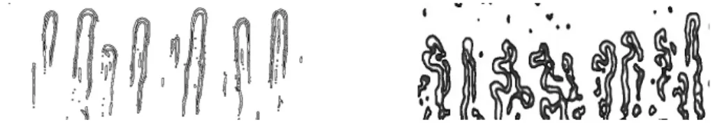
To do this, we have used the free software GIMP (see Figure 2).

Figure 2: The result of image processing of Figure 1, (Left) normal capillaries, (Right) abnormal capillaries.

3.2 Application of level set method

The level set method described in Section 2.2 is applied to the image of capillaries ob- tained in Section 3.1. Here we select the two distinctive capillaries and calculate their average curvature. We regard the shading of the image as the level set function, and perform noise removal and edge smoothing.

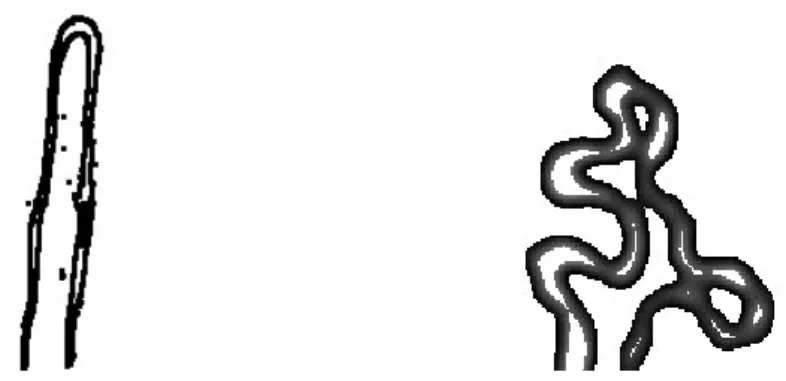
Finally, the curvature is calculated by approximating the smoothed boundary of the

capillary with circles (see (C1-3)). Figure 3 shows the images of distinctive capillaries

which are cut out from Figure 2. In the following text, the left capillary in Figure 3 is

called “normal” and the right one “meandering”. Throughout this paper, we assume that the scale size of these two pictures is the same.

Figure 3: Two distinctive capillaries, (Left) normal capillary, (Right) abnormal capillary.

We explain the procedure for calculating the average curvature of the contour of the capillaries in Figure 3. The average curvature will be defined in (C3).

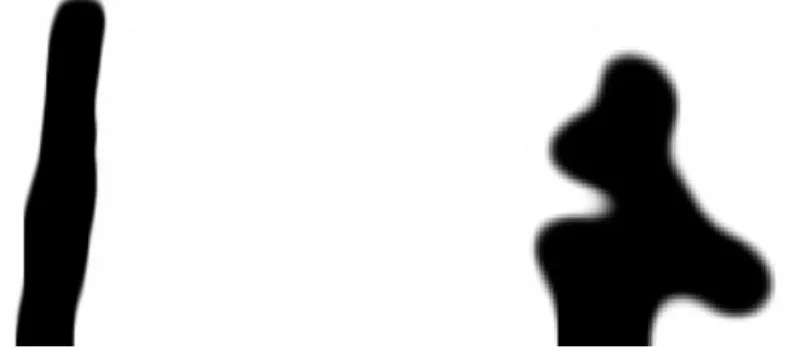
(B1) We fill the area surrounded by the capillary with black color (Figure 4).

(B2) By using the level set equation, we perform isotropic smoothing of the capillary edge.

Figure 4: The results of (B1), (Left) normal capillary, (Right) abnormal capillary.

It is known from observation that the width of the capillary wall is about 1/5 of the capillary tube. Therefore irregularities less than 1/5 of the width of the capillary are assumed to be noise. We take Figure 4 as the initial values for the level set equation, and numerical calculation is carried out 100 time steps. Then Figure 5 was obtained.

In numerical calculation, we set M = 63, K = 198 and T = K

/6.0, for the “normal”

image. Similarly, for the meandering image, we set M = 136, K = 168 and T = K

/6.0.

Figure 5: The results of (B2) (100 time steps), (Left) normal capillary, (Right) abnormal capillary.

Since the irregularities are eliminated, the curvature of the boundary can be calculated precisely. If we continue the numerical computation further more, the image is blurred.

Figure 6 shows the shape after 500 time steps of numerical calculation.

Figure 6: The results of (B2) (500 time steps), (Left) normal capillary, (Right) abnormal capillary.

Finally, the method for curvature calculation is explained. Here, we focus on two examples shown in Figure 3. In general case, a more precise definition of the average curvature will be required. There are several ways to calculate the curvature (see [5]).

This time we have used a technique that seems to be most straightforward.

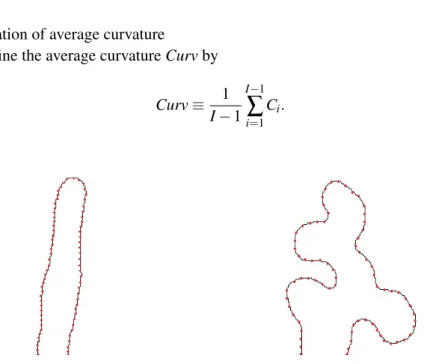
(C1) For each image of Figure 5, let a

be the left point which intersects with the bottom of the image and the capillary. We take points a

(1 ≤ i ≤ I, I ∈ N ) on the contour in the counterclockwise direction. To compensate for the difference in depth from the skin of a capillary, we define the interval between the points as the average width of the capillary ((Left) 10px and (Right) 12px)), see Figure 7. This also guarantees the scale-independence of the curvature index.

(C2) We approximate the curve (a

, a

,a

) by a circle. Let C

be the reciprocal of

the radius of the circle (1 ≤ i ≤ I − 1).

(C3) Calculation of average curvature

We define the average curvature Curv by Curv ≡ 1

I − 1

I−1

∑

C

.

Figure 7: Division points

on the contour.

3.3 Numerical results

After the above procedure, the curvature densities are obtained for the image “normal”

and “meandering” as in Table 1.

normal 1.31 × 10

meandering 2.89 × 10

Table 1: The average curvature Curv.

We can see that the introduced index curve is able to clearly distinguish the difference in the curvedness of the two capillaries, since the result for the meandering capillary is more than two times bigger than for the normal one.

4 Conclusion

Capillaries run throughout the human body and they are supplying oxygen and nutrients,

while at the same time discharging to the outside the unnecessary ingredients. This fea-

ture may change depending on the health condition. The state of the capillary can be

directly observed from the base of the nail of the middle finger. If it can be expressed in

the form of a mathematical indicator, it could be medically useful as confirmation of the

effect of a drug, etc.

In this work, we calculate average curvature of capillaries from digital images. The images contain noise and various artifacts due to capillaries and other structures appear- ing in the background. To extract the outline of the capillary, we have used the level set method. By using this method, we can smooth the boundary and eliminate noise and artifacts. This allows an effective calculation of average curvature. The results coincide with the diagnosis of the medical doctor.

In the future, we will apply this method to a large number of cases and carefully analyze the relation between our index and the medical diagnosis.

5 Acknowledgment

The authors express their appreciation to Professor Seiro Omata for his constructive sug- gestions. We also would like to express our gratitude to Professor Karel Svadlenka and Professor Elliott Ginder for their assistance.

References

[1] Yoshikazu Giga and Yun Gang Chen, “Ugoku kyokumen wo oikakete”, Nihon Hyoron-sha, (1996).

[2] H. Ishii, “Perron’s method for Hamilton-Jacobi equations”, Duke Math J.

[3] Kekkan Bijin, http://www.kekkan-bijin.com.

[4] L. C. Evans and J. Spruck, “Motion of level sets by mean curvature I”, J. Differential Geometry

(1991) 635-681.

[5] N. Ono and R. Takiyama, “On calculations of curvature of Sampled curves”, TECHNICAL REPORT OF IEICE

[6] M. G. Crandall, H. Ishii and P. L. Lions, “User’s guide to viscosity solutions of second order partial differential equations”, Bulletin of the American Mathematical Society

[7] Saburo Ogawa, “Mousaikekkanzou to rinshou”, Toriumi shobo, (1994).

[8] Azusa Suzuki, “Evaluation of the image-processing method to various noises ”, Master thesis of

Graduate School of Natural Science and Technology, Kanazawa University, (2012).