Thermal zero shift correction of strain-gage balance output in the JAXA 2m x 2m Transonic Wind Tunnel*

in the JAXA 2m x 2m Transonic Wind Tunnel ^*

Masataka KOHZAI

, Tatsurou SHIOHARA

, Makoto UENO

, Yukio KOMATSU

, Toshio KARASAWA

, Akira KOIKE

, Norikazu SUDANI

,

Yoshito GANAHA

, Mamoru IKEDA

, Atsushi WATANABE

, Tomohiro HARAGUCHI

, Muneyoshi NAKAGAWA

, Daisuke UDAGAWA

2m x 2m

香西 政孝^*1、塩原 辰郎^*1、上野 真^*1、小松 行夫^*1、唐沢 敏夫^*1、小池 陽^*1、須谷 記和^*1 我那覇 義人^*2、池田 守^*2、渡邉 篤史^*2、原口 智裕^*3、中川 宗敬^*4、宇田川 大輔^*4

I. Abstract

In the JAXA 2m x 2m Transonic Wind Tunnel, the thermal zero shift of strain-gage balance output caused by an unfavorable increase of flow temperature during a run influences the measurement accuracy of the balance. Temperature change in the balance and thermal gradients across the balance cause the thermal zero shift of the balance. Balance outputs for zero are conventionally corrected by the linear estimation from the no-wind data just before the run and the renewed no-wind data immediately after the run. In the correction method, the error increases at the beginning of the run, because the abrupt change in stagnation temperature causes balance outputs for zero to shift drastically. To reduce and correct the thermal zero shift of strain-gage balance output in force measurement, a preheating and checkpoint correction method is established. Variations of strain-gage balance output for zero are investigated during a run to confirm the effectiveness of the new method. Several series of wind tunnel tests with an ONERA-M5 calibration model and an AGARD-B calibration model are conducted to compare the new correction method with the conventional one. Results show that the error of the drag measurement from run to run is reduced to ±2 drag counts. Moreover, the new correction method is improved by using a six component internal balance with strain-gages combined with thermocouples to be applied to various kinds of models and sequences of test conditions.

Key Words: Transonic Wind Tunnel, Balance, Thermal zero shift, Data accuracy

概要

JAXA2m x 2m

力測定試験における計測精度に大きな影響を与えている。温度ドリフトを引き起こす原因としては天秤自体の温度変 化と天秤内の温度分布が考えられる。従来のドリフト補正方法では、天秤のゼロ点出力は風洞試験前のゼロ点出力と 風洞試験後のゼロ点出力を直線で結んで、その直線上の電圧をゼロ点出力とする方法であった。この補正方法では、

風洞試験開始時の気流の急激な温度上昇によって天秤のゼロ点出力が急激に変化する為、補正誤差を生じる。空気力 測定試験における温度ドリフト量を減らし、正確に補正を行う為に、予備加熱・チェックポイント補正方法を提案し た。風洞試験中の天秤のゼロ点出力変化を調べ、提案した新ドリフト補正方法の有効性を確認した。さらに、新ドリ フト補正方法と従来のドリフト補正方法の補正誤差を比較する為に

ONERA-M5

AGARD-B

2

* Received 3 December, 2007

*1 Wind Tunnel Technology Center, Institute of Aerospace Technology

*2 COSMOTEC Co., Ltd.

II. Introduction

The JAXA 2m x 2m Transonic Wind Tunnel (JTWT) has one of the largest test sections of transonic facilities in Japan, and is the only facility in this country which produces continuous transonic flows. The wind tunnel has been used for tests of most of aircraft and launch vehicles developed in Japan and for fundamental aerodynamic researches. To develop aircraft and launch vehicles with high performance, there have been more needs of wind tunnel users for high measurement accuracy of aerodynamic force, especially axial force (drag). The measurement accuracy of a six-component internal balance has to be improved to satisfy users’ needs. In the JTWT, however, an unfavorable increase of flow temperature during a run causes a thermal zero shift of strain-gage balance output, and influences the measurement accuracy of the balance.

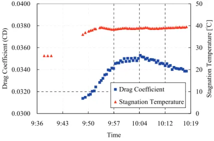
In the JTWT, drag coefficients of an ONERA-M5 calibration model (Figure 1) with an attack angle and a beta angle of 0 degree are plotted against Mach number in Figure 2. The difference between data at the beginning of the run and repeatability check data which was measured at the end of the run at Mach numbers of 0.6 and 0.7, are approximately 15 drag counts. This value corresponds to about 0.5% of the full-scale load of the drag element. Variations of stagnation temperature and drag coefficient of the model with an attack angle and a beta angle of 0 degree are shown in Figure 3, when the airflow is maintained for about 30 minutes at a Mach number of 0.8. As the stagnation temperature increases, the drag coefficient changes gradually.

These variations depend mostly on the increase of flow temperature during the run. Thus, one of the major error sources in force measurement in the JTWT is the thermal zero shift of the strain-gage balance output.

Figure 1: ONERA-M5 calibration model installed in the test section.

Figure 2: Drag coefficients of the ONERA-M5 calibration model against Mach number.

Run1972, Cart#1, P0=100kPa, Alpha=0deg, Beta=0deg

0.0200 0.0300 0.0400 0.0500 0.0600

0.50 0.60 0.70 0.80 0.90 1.00

Mach Number

Drag Co efficien t (CD)

Data

Repeatability Check Data

Figure 3: Variations of stagnation temperature and drag coefficient at the beginning of a run (M=0.8).

In continuous-flow high-speed wind tunnels, the energy generated by the main blower is usually lost in the flow circuit. In the JTWT, with the energy loss, a stagnation temperature necessarily increases by approximately 20 to 40 K, because the range of temperature control depends on a relation between a rotational speed of the main blower and cooling water exposed to the atmosphere. With the increase in the flow temperature, a model and a sting supporting the model are warmed up, so that the heat generated is gradually conducted to the model side (front) and the sting side (rear) of the balance. The temperature change of the balance and thermal gradients across the balance cause the thermal zero shift. The thermal gradients in the axial force element are severe particularly, because beams of the element are normally thin for achieving high sensitivity (Figure 4).

Figure 4: Typical balance design of the axial force element.

In 1970’s, consideration of the cryogenic concept for a European transonic wind tunnel with a large Reynolds-number range raised the question of the feasibility of force measurements with multi-component internal strain-gage balance.

At National Transonic Facility, to minimize thermal behavior differences of force balances, a gage matching technique was developed.

An individual thermal zero shift of each strain-gage was measured on a common test material. Strain-gages with nearly the same zero shifts have been matched to be bonded on the balance for bridge. Moreover, at NASA, they tried to calibrate the balance to solve the zero shift induced by temperature gradients. In the Transonic Cryogenic Tunnel at Langley, transient-temperature tests were conducted to measure the response of the balance and the variation of the temperature on the balance near the strain-gages.

Run2167, Cart#1, M=0.8, P0=100kPa, Alpha=0deg, Beta=0deg

0.0300 0.0320 0.0340 0.0360 0.0380 0.0400

9:36 9:43 9:50 9:57 10:04 10:12 10:19

Time

Dra g Coeffic ien t (CD )

0 10 20 30 40 50

Sta gna tion Te m pe ra tur e [ ℃ ]

Drag Coefficient Stagnation Temperature

Flow

Rear Front

Strain-gages

Thermal gradients cause a thermal expansion of the balance, so that a distortion of the drag element induces the zero shift of the balance output. The amount of the zero shift caused by the distortion does not depend only on thermal gradients but also on model geometry, model weight, and mass distribution.

At the Technical University of Darmstadt, a balance was build to be symmetrical to the vertical center line of the balance, so that the mechanical effect of the temperature gradient along the balance deforms the balance symmetricaly.

The beams of axial force measurement were improved to rectangular bars due to a reduction of temperature differences between the gage areas. To reduce differences in sensitivity of axial force beams, the axial force beams were designed to be a constant stress distribution in the area. In addition, the tandem axial force system was developed, with which the error signals in the fore and in the after bending beam element due to temperature gradients have the same magnitude but opposite signs. By adding the signals of the fore and the after sensors, the error signals due to temperature gradients are cancelled out. However, a standard design of a balance, which is not absolutely affected by the abrupt temperature change, has not been established. Balance temperatures are conditioned until all local balance temperatures are within 1K.

Balance calibration is performed in 20K steps. Moreover, to improve the data productivity, correction methods of thermal zero shift with the thermal gradients across the balance and analyses on the structural performance have been developed.

In the JTWT, balance outputs usually start to be measured before the thermal gradients become uniform. Because it takes long time until the thermal gradients become uniform, the data productivity is decreased remarkably. The thermal zero shifts have not been corrected exactly for several kinds of balances used in this facility, because the behavior of the thermal zero shifts vary according to balance type, model shape, and flow condition. Strain-gage outputs for zero can not be measured during the run for a few hours. Accordingly, in the JTWT, balance outputs for zero are conventionally corrected by the data on a straight line derived from the no-wind data just before the run (N-data) and the renewed no-wind data immediately after the run (R-data) as illustrated in Figure 5.

In this correction method, the error increases at the beginning of the run as shown in Figure 3, because the abrupt change in stagnation temperature causes balance outputs for zero to shift drastically. To reduce the correction error of zero shifts, the conventional data correction method has to be improved.

In this report, a new method to reduce and correct the thermal zero shift of the strain-gage balance output is proposed. To confirm the effectiveness of the new method, variations of strain-gage output for zero are investigated during runs. Several series of wind tunnel tests with the ONERA-M5 calibration model and AGARD-B model are conducted to compare the new correction method with the conventional one. Moreover, the new correction method is improved by using a six component internal balance with strain-gages combined with thermocouples to be applied to various kinds of models and sequences of test conditions.

Figure 5: Conventional data correction method.

Run Time

R-data N-data

N-data：No-wind data R-data ： Renewed no-wind data

Strain-gage output for zero Corrected output for zero

III. Facility Description

A. Wind Tunnel

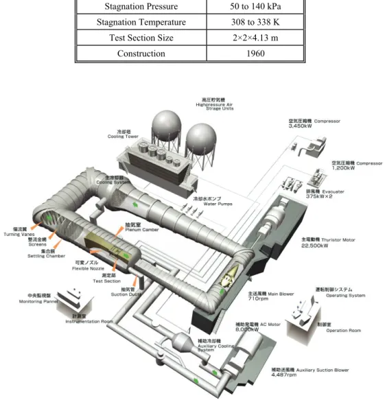
The JTWT is a closed-circuit and continuously operating facility (Figure 6). The test section is 2m wide, 2m high, and about 4m long. The Mach number range is from 0.1 to 1.4. For subsonic flows, the Mach number is controlled by the rotation of the main blower. For transonic flows, a suction blower is used to bleed the test section of airflow to avoid flow choking.

The stagnation pressure (P0) can be varied from 50 to 140 kPa, and the stagnation temperature (T0) can be varied from 308 to 338 K within the accuracy of ± 1 K. However, the range of temperature control depends on outside air temperature, because the cooling system is a heat exchanger using water. The maximum Reynolds number is about 20 million per meter (Table 1). We usually have two runs in a day. One run is for about two hours in the morning, and the other run is for about three hours in the afternoon.

Table 1: Specification of the JTWT.

Mach Number 0.1 to 1.4

Max. Reynolds Number 20×10

1/m Stagnation Pressure 50 to 140 kPa Stagnation Temperature 308 to 338 K Test Section Size 2×2×4.13 m

Construction 1960

Figure 6: Schematic of the JTWT.

B. Strain-gage balances

Internal stain-gage balances are used extensively to measure the aerodynamic loads on a test model during wind tunnel tests.

The rear side of the balance is usually supported by a sting attached to a sting-strut system in the test section. The front side of the balance is fixed in the body of the model, as the balance center corresponds to the model center. The balance is usually constructed of high-strength steel with a single piece to obtain desired stress levels in the balance itself. A Multi-component force balance uses multiple bridges to measure loads acting on the balance. A typical balance is designed with six-bridge responds to three forces and three moments, which are axial force (Fx), side force (Fy), normal force (Fz), rolling moment (Mx), pitching moment (My) and yawing moment (Mz) (Figure 7). Balance outputs are converted to forces and moments with the calibration coefficients, which are previously calculated from outputs of the bridges against different types of loads.

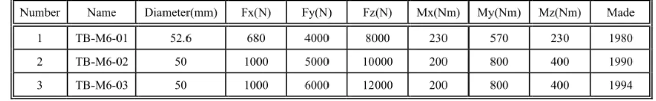
Three internal strain-gage balances are available for force measurement in the JTWT. Table 2 shows the forces and moments ranges of the balances. The balance#2 (Figure 8) and the balance#3 are almost the same configuration, but the capacity of side force and lift elements are different. The balance#1 (Figure 9) has different taper joints and relatively small ranges of six elements. One of the balances is selected according to the ranges of forces and moments which a test model senses.

Table 2: Balance list.

Number Name Diameter(mm) Fx(N) Fy(N) Fz(N) Mx(Nm) My(Nm) Mz(Nm) Made

1 TB-M6-01 52.6 680 4000 8000 230 570 230 1980

2 TB-M6-02 50 1000 5000 10000 200 800 400 1990

3 TB-M6-03 50 1000 6000 12000 200 800 400 1994

Figure 7: Balance Axis system, Forces and Moments.

Figure 8: Balance#2.

Figure 9: Balance#1.

Fz

Fy

Fx

Mx My

Mz

A N

Flow

Front Rear

Balance

C. Data acquisition system

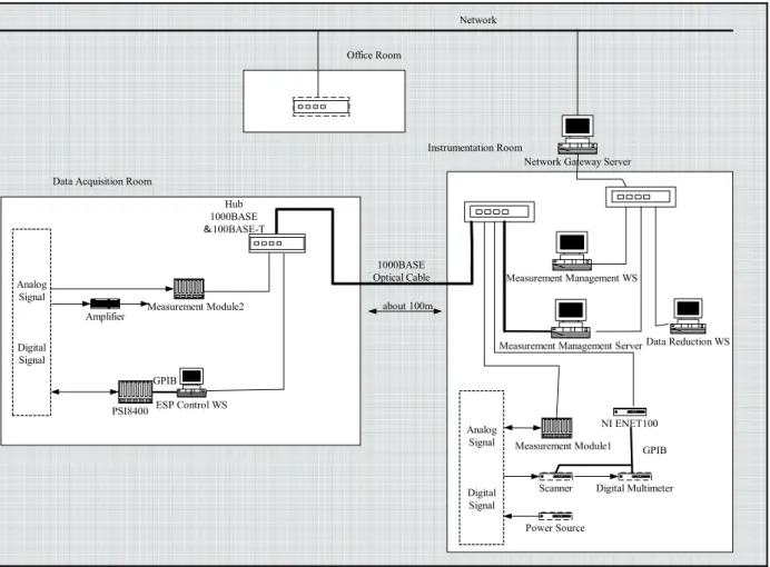
The data acquisition system consists of servers, workstations, two measurement modules, and digital voltmeters as shown in Figure 10. These are connected by IP network, which is separated from the external network by the network gateway server (NGS). The measurement managing server (MMS) manages the overall system and controls two modules with A/D and D/I interfaces, the digital voltmeters connected across a GPIB network, and the ESP control workstation. Data acquired by the measurement modules, digital voltmeters are stored in the MMS simultaneously according to the measurement request from the measurement managing workstation (MMWS). Stored data are converted to engineering units and final results in the data reduction workstation (DRWS).

Each element of strain-gage balances is provided with the DC excitation voltage by each power source (Table 3). Balance outputs and excitation voltages are measured by digital voltmeters (Table 4). These data are connected with tunnel condition and model attitudes data, which are measured by individual sensors and acquired by the measurement module1 through the D/I interface, to be stored in the MMS during a series of wind tunnel tests.

Network Gateway Server

PSI8400 ESP Control WS GPIB Data Acquisition Room

Measurement Management Server Hub

1000BASE

＆100BASE-T

Amplifier Analog

Signal

Digital Signal

Data Reduction WS 1000BASE

Optical Cable

Instrumentation Room

Measurement Module2

Analog Signal

Digital Signal Office Room

Scanner Measurement Module1 about 100m

Measurement Management WS

Digital Multimeter NI ENET100

GPIB

Power Source Network

Figure 10: Schematic of data acquisition system.

Table 3: Specification of power sources.

Output Voltage 2～13V Set Value ±0.1%F.S.

Stability ±50PPm/deg

Table 4: Specification of digital voltmeter.

Range 200mV, 2V, 20V, 200V, 1000V Integral Time 20～2000msec

Accuracy ±(0.0069 ％ of reading +3.5µV)

at Range:200mV, Integral Time:200msec

Resolution 0.1µV at Range:200mV

IV. New data correction method

The zero shift caused by the temperature change in one strain-gage is represented as follows:

( ) ^t

K R

R

g s s

⎭ Δ

⎬ ⎫

⎩ ⎨

⎧ α + β − β Δ =

where ΔR is the apparent resistance variation, R is the resistance value, α is the temperature coefficient of the resistance, K

is the gage factor, β

is the linear expansion coefficient of the spring material, β

is the linear expansion coefficient of the strain-gage, and Δ t is the temperature change. The thermal zero shift depends on the sensitivity change in the strain-gage and the difference of the thermal expansion between the strain-gage and the spring material. The temperature sensitivity and the difference have to be matched to reduce the thermal zero shift. The material and the resistance value of the strain-gage are usually selected according to the spring material. However, thermal gradients across an internal strain-gage balance cause zero shifts of balance outputs, because the thermal gradients of the beams, on which strain-gages of the drag element are pasted, cause temperature differences among four gages to form Wheatstone bridge. Furthermore, the thermal gradients across the balance induce a distortion caused by a thermal expansion of the balance.

The thermal zero shifts have not been corrected exactly, because thermal gradients depend on balance types, model shapes, and flow conditions. To reduce the correction error, balance data for aerodynamic characteristics have to be measured after thermal gradients become uniform. It takes, however, long time until the thermal gradients become uniform completely, so that the data productivity is decreased remarkably. Accordingly, the thermal zero shifts are supposed to change linearly after the thermal gradients start to become uniform, although the balance outputs for zero can not be estimated while the thermal gradients are growing. The thermal zero shifts changing linearly can be estimated precisely. Thus, a new data correction method is proposed.

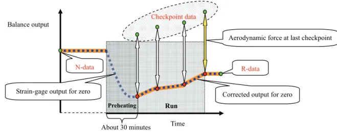
Figure 11 illustrates a typical balance output for zero and a corrected output for zero against time by the new data correction method. At the beginning of the run, to make thermal gradients of the balance uniform earlier, the airflow is maintained for approximately 30 minutes at a high Mach number. (This is called ‘preheating’.) After preheating, the strain-gage output for zero goes back to the value before the run gradually, and these data changing monotonically can be corrected easily. In the new data correction method, the zero output at the last checkpoint is supposed to be identical to the renewed no-wind data (R-data). At all of the checkpoints, balance outputs are measured under the same flow condition and in the same model attitude, so that these balance outputs should be identical to the output at the last checkpoint. The data between the checkpoints are corrected for the zero shifts by straight lines with the checkpoints.

Figure 11: New data correction method.

Run

R-data N-data

Preheating Balance output

About 30 minutes

Corrected output for zero

Aerodynamic force at last checkpoint Checkpoint data

Strain-gage output for zero

Time

V. Experimental description

Several series of wind tunnel tests are conducted with the balances to investigate the effectiveness of the new data correction method. Objectives of the wind tunnel tests are to confirm that the thermal zero shifts change monotonically after preheating and that the new correction method, which uses checkpoints and R-data, can be effective. Furthermore, we observe relations between strain-gage outputs for zero and temperature differences at both ends of the beam for axial force to estimate the thermal zero shifts precisely by the new data correction method.

A balance and a balance cover are used to observe balance outputs for zero during a run as shown in Figure 12. Figure 13 illustrates that the balance cover is supported by a sting only. The balance is not connected with the balance cover to sense no aerodynamic forces during the run. A heat insulation sheet is installed to prevent heat conduction from the sting to the balance cover. Data are acquired for three balances respectively.

Figure 12: Balance cover and balance mounted in the test section.

Figure 13: Balance cover, balance and sting description.

To observe the relation between temperatures on the balance and strain-gage outputs for zero, thermocouples are located on the balance#2 as shown in Figure 14. Thermocouples T1 and T2 are located on both sides of the beam, on which strain-gages of the axial element are pasted. Four thermocouples from T11 to T14 are located on both sides of the beams, on which strain-gages of the other elements (normal and side forces and pitching, rolling and yawing moments) are pasted. Balance data for six components and temperature data are acquired for each three balances every 15 seconds during a run.

Sting Balance

Flow

Insulating sheet

Balance cover

Figure 14: Several thermocouples located on balance#2.

VI. Experimental results

A. Results of the balance#2 and the balance#3

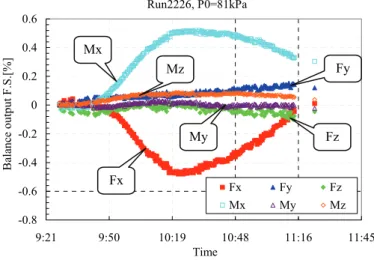
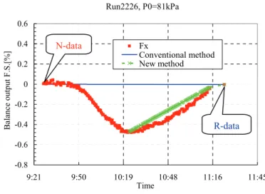
Time histories of balance#2 outputs for zero of all elements are shown in Figure 15. Outputs of Fx and Mx change drastically during preheating and go back to zero after preheating. Outputs of the other elements vary gradually, and their variations are 0.2% or less. For these elements, the conventional data correction method is acceptable. However, when the conventional correction method is applied to Fx data, the maximum error reaches 0.5%. Balance outputs should be acquired after the peak of zero shifts of the balance to make the correction simpler (Figure 16). When the Fx data are corrected by the new correction method, the error can be decreased to 0.05% or less. The new data correction method, therefore, has proved to be very effective.

Figure 15: Variations of balance outputs for zero of all elements during the run (Balance#2).

Flow

T11 T12

T13 T14

T2

T1

Run2226, P0=81kPa

-0.8 -0.6 -0.4 -0.2 0 0.2 0.4 0.6

9:21 9:50 10:19 10:48 11:16 11:45

Time

Balance output F.S.[%]

Fx Fy Fz

Mx My Mz

Fy

Fz Mx

My Mz

Fx

Figure 16: Balance outputs for zero of drag element during the run (Balance#2).

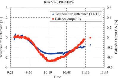
Time histories of stagnation temperature and temperatures on the balance are plotted in Figure 17. While the stagnation temperature increases drastically, all of the measured temperatures on the balance increase gradually. To observe relations between thermal gradients across the balance and thermal zero shifts of the drag element, time histories of temperature differences between T1 and T2 on both sides of the beam for the drag element and drag outputs are plotted in Figure 18. The temperature differences between T1 and T2 change similarly to the drag outputs. This fact implies that the output for zero can be estimated from the temperature difference. Correlations between temperature differences and outputs for zero are investigated with a temperature-controlled bath by providing the balance with various kinds of temperature differences condition. In the result, a function to correct thermal zero shifts from temperature differences, however, can not be calculated precisely, because thermal zero shifts and measured temperature differences do not change quite simultaneously, and not only temperature differences in this part, but also thermal gradients on the whole balance affect on thermal zero shifts. Thus, although thermal zero shifts can not be corrected only with the temperature differences, temperatures on the balance during the wind tunnel tests need to be monitored to confirm that thermal gradients become uniform.

A series of similar wind tunnel tests is conducted with balance#3. Thermal zero shifts and thermal gradients of balance#3 change similarly to those of balance#2, because these two balances have almost the same configuration.

Figure 17: Variations of stagnation temperature and thermocouples during the run (Balance#2).

Run2226, P0=81kPa

-0.8 -0.6 -0.4 -0.2 0 0.2 0.4 0.6

9:21 9:50 10:19 10:48 11:16 11:45

Time

Balance output F.S.[%]

Fx Conventional method New method

R-data N-data

Run2226, P0=81kPa

10 15 20 25 30 35 40

9:21 9:50 10:19 Time 10:48 11:16 11:45

Balance Temperature [℃]

T1 T2

T11 T12

T13 T14

T0 T12, T14

T11, T13

T1

T2

Figure 18: Relation between temperature difference and balance output for zero (Balance#2).

B. Results of the balance#1

Time histories of balance#1 outputs for zero of all elements are shown in Figure 19. Outputs of the force elements (Fx, Fy, and Fz) shift by 0.2% or more, while outputs of the moment elements (Mx, My, and Mz) change gradually. Outputs of all components for the balance never go back to zero during the run, although the airflow is maintained for 30 minutes at a Mach number of 0.9. Thus, the correction error is 0.05% or less, in the case where the conventional method is applied to Fx data (Figure 20). When the Fx data are corrected by the new correction method, the error can be decreased further.

Figure 19: Variations of balance outputs for zero of all elements during the run (Balance#1).

Run2226, P0=81kPa

-3 -2 -1 0 1 2 3

9:21 9:50 10:19 10:48 11:16 11:45

Time

Temperature Difference [℃]

-0.6 -0.4 -0.2 0 0.2 0.4 0.6

Balance Output F.S.[%]

Temperature difference (T1-T2) Balance ourput Fx

Run2314, P0=81kPa

-0.4 -0.2 0 0.2 0.4 0.6 0.8 1

9:21 9:50 10:19 10:48 11:16 11:45

Time

Balance Output F.S.[%]

Fx Fy Fz Mx My Mz

Fy

Fx Fz

Mx My

Mz

Figure 20: Balance outputs for zero of drag element during the run (Balance#1).

To investigate temperatures on balance#1 during the run, thermocouples are located on balance#1 as shown in Figure 21.

Thermocouples T1 and T2 are located on both sides of the beam, on which strain-gages of the axial element are pasted. Time histories of stagnation temperature and temperatures on the balance are plotted in Figure 22. While the stagnation temperature increases drastically, all of the measured temperatures on balance#1 increase gradually. To observe relations between thermal gradients across the balance and thermal zero shifts of the drag element, time histories of temperature differences between T1 and T2 on both sides of the beam for Fx and balance outputs of Fx are plotted in Figure 23. The temperature difference (T1-T2) decreases gradually and has a peak just before the end of the run, although the airflow is preheated at the same Mach number as balance#2. It takes a longer time for temperatures to be identical in various locations of the balance, because balance#1 has a larger thermal capacity than balance#2. Moreover, the structure of the axial force element in balance#1 is different from that in balance#2. Strain-gages for Fx are pasted on both front beams and rear beams in balance#2 as shown in Figure 4, while in balance #1, both front beams and rear beams are thinner than those of balance#2, and there is only one beam for the axial force in the center as shown in Figure 24. Accordingly, thermal gradients across balance #1 do not become uniform easily.

Figure 21: Several thermocouples located on Balance#1.

The thermal zero shift of the drag element never goes back to zero during the run, although the temperature difference (T1-T2) has the peak just before the end of the run. This fact means the thermal zero shift is not caused only by the temperature difference but also by the distortion of the beam. The maximum value of the thermal zero shift is only as half as the peak value

Flow

T3

T4 T1

T2 T5

T6 T13 T14

T11 T12 Run2314, P0=81kPa

-0.4 -0.2 0 0.2 0.4 0.6 0.8 1

9:21 9:50 10:19 10:48 11:16 11:45

Time

Balance Output F.S.[%]

Fx

Conventional method New method

R-data

N-data

of the zero shift of balance#2, and a sensitivity of the thermal zero shift to the temperature difference is also as half as that of balance#2. It seems that they are partly attributed to the structure difference of the axial force element. Thus, it is better to use balance#1 with the conventional correction method in the case where the duration of the run is not so long, and the data productivity is given to priority more than the data accuracy. In the case where preheating time is secured sufficiently, thermal zero shifts can be corrected by the new method precisely even if either balance is used.

Figure 22: Variations of stagnation temperature and thermocouples during the run (Balance#1).

Figure 23: Relation between temperature difference and balance output for zero (Balance#1).

Figure 24: Configuration of axial force element (Balance#1).

Run2314, P0=81kPa

-3 -2 -1 0 1 2 3

9:21 9:50 10:19 10:48 11:16 11:45

Time

Temperature Difference [℃]

-0.6 -0.4 -0.2 0 0.2 0.4 0.6

Balance Output F.S.[%]

Temperature difference (T1-T2) Balance output Fx

Flow

Strain-gages Run2314, P0=81kPa

10 15 20 25 30 35 40

9:21 9:50 10:19 10:48 11:16 11:45

Time

Balance Temperature [℃]

T1 T2

T11 T12

T13 T14

T0 T12, T14 T11, T13

T1

T2

VII. Application of the new correction method to the calibration model

A series of wind tunnel tests with the ONERA-M5 calibration model and balance#2 is conducted to compare the new correction method with the conventional one. For several runs at a Mach number of 0.74, lift coefficients (CL) are plotted against drag coefficients (CD) in Figure 25. At a lift coefficient of 0.0, the drag coefficient differences between the data corrected by the conventional method and the data corrected by the new method are significant. The repeatability in the three sets of data corrected by the new method is within a few drag counts. The accuracy of force measurement has improved remarkably. The three sets of data acquired after preheating and corrected by the conventional method are scattered, and different from the data corrected by the new method significantly. It can be seen that the checkpoint correction has to be applied to the data acquired after preheating. Drag coefficients of the ONERA-M5 calibration model with an attack angle and a beta angle of 0 degree are plotted against Mach number in Figure 26. The difference between two correction methods is meaningful.

Particularly, the correction error with conventional method occurs at Mach numbers of 0.7 and 0.74, at which the balance starts to be heated as the increase in the stagnation temperature. The repeatability among four runs with the new method is also better than that with the conventional method. Thus, the new method is proved to be effective.

Figure 25: Comparison of the new method with the conventional method at a Mach number of 0.74.

Figure 26: Comparison of the conventional method with the new method for drag coefficients.

Cart#1, P0=100[kPa], Alpha=0[deg], Beta=0[deg]

0.01 0.02 0.03 0.04 0.05 0.06

0.5 0.6 0.7 0.8 0.9 1

Mach Number

Drag Coefficient (CD)

Run#2163 (Conventional method) Run#2164 (Conventional method) Run#2165 (New method) Run#2166 (New method) Run#2167 (New method) Run#2168 (New method)

Cart#1, M=0.74, P0=100[kPa]

-0.20 -0.10 0.00 0.10 0.20 0.30 0.40 0.50 0.60 0.70

0.010 0.015 0.020 0.025 0.030 0.035 0.040 0.045 0.050 0.055 0.060 0.065 0.070

Drag Coefficient (CD)

Lift Coefficient (CL)

Run#02163(Conventional method) Run#02165(New method) Run#02166(New method) Run#02167(New method)

Run#02165(Preheated, Conventional method) Run#02166(Preheated, Conventional method) Run#02167(Preheated, Conventional method)

VIII. Improvement of the new correction method

By using the new correction method (preheating and checkpoint correction method), the accuracy of force measurement has been improved remarkably. When this method is applied to various kinds of models and sequences of test conditions, however, two problems would be mainly occurred. To solve these problems, operation and correction method have to be improved.

One problem is that, appropriate preheating time and thermal zero shifts after preheating for any model need to be grasped at any runs. Preheating has to be continued until thermal gradients become uniform. Variations of balance temperatures after preheating should be measured, because balance temperatures are the only way to estimate variations of balance outputs for zero during the run. Thus, to measure temperature distributions of a balance installed in a model during the run, a new balance (Balance#4) is made with strain-gages combined with thermocouples as shown in Figure 27, Figure 28, and Table 5. Fx and My elements, which are likely to be influenced by the thermal zero shift, are used strain-gages with thermocouples. The shape of Balance#4 is almost similar to Balance#1.

Figure 27: Balance#4 made with strain-gages combined with thermocouples.

Figure 28: Locations of strain-gages with thermocouples at an axial force element.

Table 5: Specification of Balance#4.

Number Name Diameter(mm) Fx(N) Fy(N) Fz(N) Mx(Nm) My(Nm) Mz(Nm) Made

4 TB-M6-04 52.6 670 4000 8000 226 565 226 2006

The balance and an AGARD-B model are used to observe variations of balance outputs of Fx, balance temperatures from T1 to T4, and stagnation temperature during a run as shown in Figure 29. For balance outputs of Fx, data during preheating and checkpoint data at a Mach number of 0.9 with an attack angle and a beta angle of 0 degree are plotted. While the stagnation temperature increases drastically, the upstream strain-gage temperatures T1 and T4 are increasing. The downstream strain-gage temperatures T2 and T3 increase after some delay. Thermal gradients become uniform gradually. The increase in balance outputs of Fx becomes gradual after the thermal gradients become uniform, although outputs of Fx change drastically at the beginning of

Flow

T3

T1 T4

T2 Thermocouple

Strain-gage

preheating. It is found that the wind tunnel should be preheated until temperature differences between the upstream and downstream strain-gages become uniform and until variations of balance outputs of Fx become uniform. After preheating, thermal gradients do not change significantly, because the test is conducted within a Mach number range from 0.8 to 0.9.

Accordingly, balance outputs for zero do not change drastically. Besides, stagnation temperature during all the run needs to be controlled to keep thermal gradients constant after preheating. Although the stagnation temperature previously increases gradually because of the cooling system performance, the stagnation temperature can be controlled by setting the stagnation temperature higher than before.

Relations between changes in Mach number and changes in temperature distributions of the balance are investigated closely as shown in Figure 30. The temperature distributions on the balance change steadily according to the changes in the Mach number and the stagnation temperature. The reaching balance temperatures correspond to adiabatic wall temperatures (T

) approximately. T

on turbulent boundary layer is given by the following equations:

∞

∞

⎭ ⎬ ⎫

⎩ ⎨

⎧ + γ −

= M T

2 ) 1 0 ( r 1

T

3 1

Pr ) 0 ( r =

where γ is the ratio of specific heat, M

is the freestream Mach number, T

is the freestream static temperature, and Pr is the Prandtl number. Model surfaces except for a front edge and most part of sting surfaces are warmed up by the airflow, so that their temperatures change into T

approximately. Temperature distributions of a balance attached to both the model and the sting also change into T

gradually. Thus, stagnation temperature should be controlled to keep T

constant according to changes in Mach numbers as lines shown in Figure 31. Accordingly, thermal zero shifts caused by changes in thermal gradients can be reduced further. Moreover, a run need to be conducted in a limited Mach number range, because stagnation temperature can not be controlled immediately for a drastic change in Mach number (for instance, from 0.9 to 0.4). Balance data for aerodynamic characteristics in a wide Mach number range should be acquired at a few runs in limited Mach number ranges.

Figure 29: Variations of balance output Fx, balance temperature T1 to T4, and stagnation temperature during a run.

Run2870, P0=100kPa, AGARD-B Model

30 35 40 45 50 55

13:12 13:40 14:09 14:38 15:07 15:36 16:04 16:33 17:02 Time

T emp er at ur e [ ℃ ]

-0.226 -0.224 -0.222 -0.22 -0.218 -0.216

B ala nc e our put Fx [ m V ]

T1 T2 T3 T4

T0 Fx (M=0.9, Alpha=0) T1, T4

T2, T3

Figure 30: Relations among Mach numbers, balance temperatures, and adiabatic wall temperatures

Figure 31: Relations between stagnation temperature and Mach number to keep adiabatic wall temperature constant.

Another problem is that a correction error caused by variations of checkpoint data need to be reduced, because in the checkpoint correction method, balance outputs for zero are estimated by using the assumption that all checkpoint data are supposed to be the same aerodynamic force data. At a Mach number of 0.98, to which drag coefficients are highly sensitive, balance outputs of Fx after preheating are scattered within a range of 6 µV as shown in Figure 32. The variation of the drag coefficient corresponds to the time fluctuation of freestream Mach number in Figure 33, so that the variation of the balance outputs of Fx after preheating must be caused by the fluctuation of the Mach number. The fluctuation of Mach number can not, however, be reduced, because Mach numbers are generally well controlled within a range of 0.001. Accordingly, fluctuations of Mach number cause correction errors of thermal zero shifts, when a Mach number, to which aerodynamic forces are highly sensitive, is selected as a checkpoint Mach number.

To reduce the correction errors, the sensitivity of balance outputs to Mach numbers at a checkpoint Mach number is calculated from a few balance outputs. Each checkpoint data can be corrected for fluctuations of Mach number with the sensitivity.

Sensitivities are supposed to be calculated from data sets acquired at the end of the run, because thermal zero shifts hardly change at the end of the run. Figure 34 shows that by using checkpoint data corrected with the sensitivity, the correction error

Run2870, P0=100kPa, AGARD-B Model

45 46 47 48 49 50 51 52

13:12 13:40 14:09 14:38 15:07 15:36 16:04 16:33 17:02 Time

T emp er at ur e [ ℃ ]

0.7 0.75 0.8 0.85 0.9 0.95 1 1.05

M ach n umb er

T1 T2 T3

T4 T0 Taw

Taw+2.0 Mach

Adiabatic wall temperature (Taw)

47 48 49 50

0.6 0.65 0.7 0.75 0.8 0.85 0.9 0.95 1

Mach number

Stagnation temperature (T0) [℃]

Taw = 45.0℃

Taw = 44.8℃

Taw = 44.6℃

Taw = 44.4℃

Taw = 44.2℃

Taw = 44.0℃

Taw = 43.8℃

T1, T4 T2, T3

of thermal zero shifts can be reduced to the half or less. Moreover, when tests are conducted in such Mach numbers, sensitivities of each Mach number should be calibrated in advance.

Figure 32: Variations of balance outputs Fx at a Mach number of 0.98, to which drag coefficient is highly sensitive.

Figure 33: Relations between variations of drag coefficient and time fluctuations of Mach number.

Figure 34: Improvement of drag coefficient variations by using checkpoints data corrected with sensitivity to Mach number.

Run2869, P0=100kPa, M=0.98, Alpha=0deg, Beta=0deg, AGARD-B Model

0.0367 0.0368 0.0369 0.0370 0.0371 0.0372 0.0373 0.0374 0.0375 0.0376 0.0377

0.979 0.9795 0.98 0.9805 0.981

Mach number

Dr ag Co eff ici en t ( C D)

Checkpiont correction with sensitivity to Mach number

Checkpoint correction only

Run2869, P0=100kPa, M=0.98, Alpha=0deg, Beta=0deg, AGARD-B Model

0.0367 0.0368 0.0369 0.037 0.0371 0.0372 0.0373 0.0374 0.0375 0.0376 0.0377

11:20 11:21 11:22 11:23 11:24 11:25 11:26 11:27 11:28 Time

Drag Co eff icien t (CD)

0.9790 0.9792 0.9794 0.9796 0.9798 0.9800 0.9802 0.9804 0.9806 0.9808 0.9810

Ma ch num be r

CD Mach Run2869, P0=100kPa, AGARD-B Model

10 15 20 25 30 35 40 45 50 55

9:36 9:50 10:04 10:19 10:33 10:48 11:02 11:16 11:31 Time

T emp eratu re [ ℃ ]

-0.344 -0.342 -0.340 -0.338 -0.336 -0.334 -0.332 -0.330 -0.328 -0.326

B ala nc e output Fx [ m V ]

T1 T2 T3 T4

T0 Fx (M=0.98, Alpha=0) T1, T4

T2, T3

IX. Conclusion

To improve the force measurement accuracy, a preheating and checkpoint correction method to reduce and correct the thermal zero shift of the balance has been proposed. The application of preheating results in a monotonic change in the strain-gage output for zero. The output for zero, therefore, can be corrected easily, and the checkpoint correction is proved to be effective for the reduction of drag measurement error. Furthermore, there is a correlation between the strain-gage output for zero and the temperature difference at both ends of the beam for the drag element.

The new correction method is improved to be applicable to various kinds of models and sequences of test conditions. To measure temperature distributions of a balance installed in a model during a run, a new balance is made with strain-gages combined with thermocouples. It is found that preheating should be continued until temperature differences between upstream and downstream gages become uniform and until variations of balance outputs become uniform. After preheating, temperature distributions on the balance gradually change into approximately adiabatic wall temperature (T

) according to changes in Mach numbers and stagnation temperature, because temperatures of the model surface and most part of the sting surface change into T

. Stagnation temperature should be controlled to keep adiabatic wall temperature constant according to changes in Mach numbers. Furthermore, to reduce the correction error caused by variations of checkpoint data, the sensitivity of balance outputs to Mach numbers at a checkpoint Mach number is calculated from a few balance outputs, and each checkpoint data are corrected for the fluctuation of the Mach number with the sensitivity. Results in several series of wind tunnel tests with an ONERA-M5 calibration model and an AGARD-B calibration model, show that the repeatability of the force measurement from run to run is improved from approximately ±15 drag counts with the conventional method to ±2 drag counts or less with the new correction method.

X. Acknowledgments

The authors would like to thank Mr. Nobuhiro Toda, Mr. Masamitsu Suzuki, and Mr. Seizou Suzuki in the Transonic Wind Tunnel Section for their help in conducting experiments.

XI. References

1. K. Hufnagel, and B. Ewald: Force Testing with Internal Strain Gage Balances, AGARD-R-812, 1997

2. Alice T. Ferris: Cryogenic Strain Gage Techniques Used in Force Balance Design for the National Transonic Facility, NASA TM-87712, 1986

3. Richmond P. Boyden, Alice T. Ferris et al.: Aerodynamic Measurements and Thermal Tests of a Strain-Gage Balance in a Cryogenic Wind Tunnel, NASA TM-89039, 1987

4. J. F. Baljeu: Development of a multi-component internal strain-gauge balance for model tests in a cryogenic wind tunnel, NLR TR 88157 U, 1988

5. R. Rebstock: Development of Correction Procedure for Signals of Cryogenic Balances, AGARD-R-812, 1997

6. James Hereford, Peter A. Parker, and Ray D. Rhew: Impact of Thermal Gradients on Wind Tunnel Force Measurements, AIAA-99-0309

7. Frank W. Steinle, Jr.: Calibration of Strain-Gage Balance for Thermal Effects, AIAA 2002-0882

8. R. Karkehabadi, R. D. Rhew and D. J. Hope: Study and Analyses on the Structural Performance of a Balance, NASA TM-213263, 2004

9. K. Suzuki, S. Nakamura and T. Fujita: Thermal zero shift correction method in the NAL 2mx2m transonic wind tunnel, National Aerospace Laboratory, Report TM-432, 1981

10. W. Lance Richards: A New Correction Technique for Strain-Gage Measurements Acquired in Transient-Temperature

Environments, NASA Technical Paper 3593, 1996