A Study of Adaptation Luminance for Mesopic Photometry

(1)

A Study of Adaptation Luminance for Mesopic Photometry

January 2017

Doctor of Engineering

Tatsukiyo Uchida

Toyohashi University of Technology

　　（薄明視測光のための順応輝度に関する研究）

(2)

(3)

Abstract

To measure light and lighting, current practice always uses the spectral luminous eﬃciency function, V (λ), which represents the visual perception by light at equal power for each wavelength. However, the V (λ) was developed only based on the sensitivity of the central field of view that adapts to higher light levels. It is known that the peripheral field of view shifts its spectral sensitivity to shorter wavelengths in darker light levels, called the mesopic range. Current lighting practice is not optimized for the light levels.

The recommended system for mesopic photometry published by the Commis- sion Internationale de l’Éclairage (CIE) provides the spectral luminous eﬃciency function, V

mes;m

(λ), the shape of which changes depending on the adaptation luminance in the mesopic range. The system could open the door to more energy- eﬃcient lighting. According to an estimate in this study, 10 % to 40 % energy saving could be possible. However, lack of methods to determine the adaptation luminance for particular lit scenes prevents the system being implemented.

This study aims to propose an adaptation field definition, where the average luminance suﬃciently correlates to the adaptation luminance, for the mesopic photometry system implementation. The first question is whether the peripheral adaptation depends only on the local luminance or on the global average luminance in the field of view. A series of vision experiments revealed that the local luminance is the dominant factor even for the mesopic and peripheral adaptation. However, the surrounding luminance also slightly aﬀects the adaptation and its impact may be significant when high-luminance sources exist in lit scenes.

Further vision experiments were conducted to characterize the surrounding lu-

minance eﬀect. According to the experiments, it can be considered as the veiling

luminance caused by stray light in eyes. However, existing veiling luminance mod-

els do not agree with the experimental results. This study proposes a new model

that is suitable to predict the peripheral veiling luminance in the mesopic range.

(4)

the luminance distribution, by taking both the surrounding luminance eﬀect and the eye movements into account. The simulation results show good agreement with the empirical data acquired in this study. By applying the simulation method to real road luminance distributions, adaptation field candidates were tested. Ac- cording to the analysis, the adaptation field can be defined as the design area of the lighting (i.e. road surface) for typical road lighting. Limitations of this proposal are also discussed.

For rigorous field photometric measurements with the mesopic photometry sys- tem, special luminance meters that are not widely available at present are needed.

To avoid use of such instruments, this study proposes simplified measurement methods. Since road surface spectral reflectance variations cause some errors with the proposed methods, the error was analyzed with real road surface spectral re- flectance data. The analysis shows that a proposed method with a correction can measure the mesopic quantities accurately enough only with conventional instru- ments and source spectral power distribution data.

The proposed adaptation field definition and the field measurement method en- able the mesopic photometry implementation to typical road lighting. These allow more energy-eﬃcient lighting design for the applications. For more general adap- tation field definitions, further field luminance distribution examples are needed.

However, once such data is available, the methodology established in this study

could give comprehensive solutions.

(5)

Acknowledgment

First and foremost I would like to thank Dr. Yoshi Ohno, a NIST Fellow. I had done most of the work as a NIST guest researcher hosted by him. I learned from him how I should analysis problems on a deeper scientific level. He also guided me through the CIE activities and taught me how fundamental researches are important for such activities. Without his advice, I would not have been able to overcome the numerous obstacles, which I had faced throughout my research.

I would like convey my deep appreciation to Prof. Shigeki Nakauchi for his sincere support for drafting and completing this dissertation. Ever since I openly aspired to a doctoral degree, he had consistently been a strong supporter. I am also grateful to the chair and a co-chair of my dissertation committee, Prof. Shigeru Kuriyama and Prof. Jun Miura, for their patience and beneficial discussions.

I would also like to express my gratitude to the members of the Japanese Solid- State Lighting Strategic Committee in 2010: Dr. Tetsuji Takeuchi, Mr. Masanori Doro, Dr. Takayoshi Fuchida, and Mr. Ken-ichi Suzuki. Not only was my research project at NIST a part of their grand plan, but also I would not have been able to start up and finish my project without their support. My experiments were designed based on Dr. Takeuchi’s works. Dr. Fuchida introduced me to Dr. Ohno and recommended that I should take a doctorate degree. Mr. Suzuki’s suggestion was the most significant factor when deciding on the subject of the project.

My sincere thanks also go to members of Optical Radiation Group at NIST, including Mr. Yuqin Zong, Dr. Cameron Miller, Dr. Maria Nadal, Dr. George Eppeldauer, and Dr. Vyacheslav Podobedov for their great support, advice, and friendship. I learned a plenitude of state-of-the-art photometry from them. They also assisted me to get accurate measurements, which underpinned the work.

Thank you as well to guest researchers that shared a NIST oﬃce room with

me: Dr. Hideyoshi Horie, Dr. Arno Keppens, Dr. Kenji Godo, Dr. Christophe

Martinsons, Dr. Irena Fryc, Mr. Tokihisa Kawabata, and Dr. Haiping Shen. Their

(6)

their friendship made my NIST research life delightful.

I am also grateful to the members of JCIE JTC-1 mirror committee: Prof.

Miyoshi Ayama, Prof. Yukio Akashi, Prof. Naoya Hara, Mr. Toru Kitano, Mr.

Yasuhiro Kodaira, Ms. Tomoko Kotani, Dr. Takako Kimura, Dr. Tomokazu Hagio, and Mr. Kazutoshi Sakai. The committee’s constructive discussions were crucial to the completion of the simulation research in Chapter 5.

My sincere appreciation also goes to great scientists in the CIE, such as Dr.

Teresa Goodman, Prof. Liisa Halonen, Dr. Marjukka Puolakka, Prof. Ronnier Luo, Dr. Ken Sagawa, Dr. Hiroshi Shitomi, and Prof. Janos Schanda. They inspired and encouraged me with their commentary. However, I am extremely saddened that Prof. Schanda passed away and we can no longer have our discussions anymore.

I am especially grateful to all Panasonic personnel that supported my work. The directors at the R&D Center of Panasonic’s Lighting Business Unit, Mr. Kazuo Kamata, Mr. Katsumi Sato, Mr. Takayuki Imai, and Mr. Masaaki Isoda, approved me to pursue the project. Mr. Shinji Noguchi, Mr. Nobumichi Nishihama, Mr.

Wataru Tanaka, Mr. Koji Noro, Dr. Ken-ichiro Tanaka, and Mr. Masato Ohnishi also generously allowed me to spend time for the work. If Mr. Toshihiko Sakaguchi had not recommended me for the project, I would not have had the opportunity to engage in such meaningful work. Without Mr. Atsunori Okada’s logistic work, I would not have been able to finish my project successfully. Mr. Makoto Yamada accepted that I left his team for the project. Mr. Takashi Saito and Dr. Hiroki Noguchi also gave me both professional and personal advice.

Most of this work is a part of a project funded by the New Energy and Industrial Technology Development Organization (NEDO). I really appreciate NEDO and the Ministry of Economy, Trade and Industry for funding the project.

Lastly, I would like to thank my dearest family for all of their love and encour-

agement. When I decided to stay in the United States for the duration of the

project, they agreed to come along with me even though they knew it would be

challenging for them. I was relieved when my sons, Tamon and Ryojun, were able

to overcome those challenges and adapt well to their new environment. Even after

we returned to Japan, they allowed me to spend time in private to write. Most of

all, I am thankful for my loving, supportive, encouraging, and patient wife, Asuka,

whose faithful support kept me going. Thank you.

(7)

List of Figures

1.1 Spectral luminous eﬃciency functions . . . . 3 2.1 A photometer for visual photometry . . . . 7 2.2 A physical detector of optical radiation . . . . 8 2.3 The photopic and scotopic spectral luminous eﬃcacy functions . . 10 2.4 Spectral sensitivities of dark-adapted foveal cones, peripheral rods,

and peripheral cones (Wald, 1945) . . . . 11 2.5 Mesopic spectral luminous eﬃciency at 10

^◦

eccentricity (Walters

and Wright, 1942) . . . . 12 2.6 The mesopic spectral luminous eﬃcacy functions . . . . 16 2.7 Estimated energy-saving eﬀect by lighting design with the mesopic

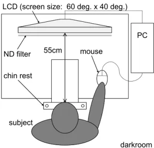
photometry system . . . . 18 3.1 Depiction of the experimental set-up for the adaptation pattern

experiment and the adaptation background luminance experiment 24 3.2 Spectral power distributions for white, red and blue stimuli pre-

sented on the display . . . . 24 3.3 Adaptation patterns and task patterns used for the adaptation pat-

tern experiment . . . . 25 3.4 The mean luminance contrast detection thresholds for all subjects

in the adaptation pattern experiment . . . . 30 3.5 The mean luminance contrast detection thresholds normalized for

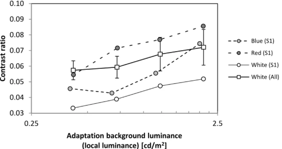
the Condition A thresholds in the adaptation pattern experiment 30 3.6 The contrast detection thresholds in the adaptation background

luminance experiment . . . . 33 3.7 Conceptual diagrams for how to determine the eﬀective adaptation

luminance . . . . 35

(12)

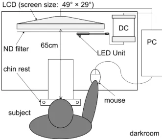
4.2 Adaptation patterns and the task pattern used for the point-source intensity experiment . . . . 45 4.3 Magnification of an adaptation pattern and the task pattern . . . 45 4.4 Schematic elevation of the LEDs, the jig and the LCD for the point-

source position experiment . . . . 48 4.5 Adaptation patterns and a task pattern used for the point-source

position experiment . . . . 49 4.6 Adaptation patterns and a task pattern used for the uniform ex-

periment . . . . 50 4.7 The mean luminance contrast detection thresholds for all subjects

for a point-source position of 7

^◦

in the point-source intensity exper- iment . . . . 52 4.8 The mean luminance contrast detection thresholds for all subjects

for a point-source position of 15

^◦

in the point-source intensity ex- periment . . . . 52 4.9 The mean luminance contrast detection thresholds for all subjects

for a point-source position of 30

^◦

in the point-source intensity ex- periment . . . . 53 4.10 The mean luminance contrast detection thresholds for all subjects

for the near-point-source conditions and associated reference con- ditions in the point-source position experiment . . . . 54 4.11 The mean luminance contrast detection thresholds for all subjects

for the far-point-source conditions and associated reference condi- tions in the point-source position experiment . . . . 54 4.12 The mean luminance contrast detection thresholds for repeated tri-

als with one subject in the uniform experiment . . . . 56 4.13 The eﬀective adaptation luminances determined from the experi-

mental results and the models, as functions of the vertical illumi- nance from the point source . . . . 58 4.14 The surrounding luminance eﬀects from the experiments and the

veiling luminance predicted with the models, per one lux of vertical

or normal illuminance from the point source . . . . 63

(13)

5.1 The object coordinate system and the retinal coordinate system . 67 5.2 Comparisons of the simulated adaptation luminance and the eﬀec-

tive adaptation luminance in the point-source intensity experiment 74

5.3 Luminance distribution examples: Sidewalks in urban area . . . . 76

5.4 Luminance distribution examples: Walkways in a park . . . . 76

5.5 Simulated adaptation luminance with small EM . . . . 78

5.6 Simulated adaptation luminance with midsize EM . . . . 78

5.7 Simulated adaptation luminance with large EM . . . . 79

5.8 Ratio of the simulated adaptation luminance for non-HDR LD to that for the HDR LD . . . . 81

6.1 The spectral reflectance of road surfaces in good condition . . . . 88

6.2 The spectral reflectance of damaged road surfaces . . . . 88

6.3 The spectral reflectance of fresh yellow and white paint on a road 88 6.4 The SPDs of the light sources used in the error simulation . . . . 89

6.5 Simulated error distribution for the Adaptation SPD method with MH lighting . . . . 91

6.6 Simulated error distribution for the Adaptation SPD method with HPS lighting . . . . 91

6.7 Simulated error distribution for the Adaptation SPD method with LED lighting . . . . 92

6.8 Simulated error distribution for the Source SPD method with MH lighting . . . . 93

6.9 Simulated error distribution for the Source SPD method with HPS lighting . . . . 93

6.10 Simulated error distribution for the Source SPD method with LED lighting . . . . 94

6.11 Correction factors for various light sources with spectral reflectance data of asphalt and concrete . . . . 96

6.12 Simulated error distribution for the corrected Source SPD method with LED lighting . . . . 96

6.13 Simulated errors in the mesopic luminance calculated with the Source

SPD method in some adaptation fields illuminated with LEDs and

HPS . . . . 98

(14)

(15)

List of Tables

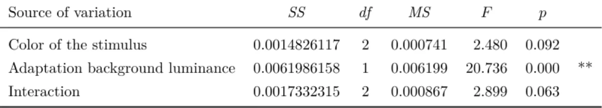
3.1 Two-way ANOVA for Conditions A, B and C in the adaptation pattern experiment . . . . 32 3.2 Two-way ANOVA for Conditions A and D in the adaptation pattern

experiment . . . . 32 3.3 The photopic eﬀective adaptation luminance and the mesopic test

luminance calculated from the experimental data and models . . . 36 4.1 The impact of the surrounding luminance eﬀect on the mesopic

luminance of a test object for the CIE road lighting classes . . . . 60

5.1 Extent of the eye movements in existing studies . . . . 68

(16)

(17)

1 Introduction

1.1 Background

The role of lighting is facilitating human visual tasks and creating comfortable visual atmosphere. To design, specify, install, and maintain lighting, light needs to be dealt quantitatively so that the quantities can correspond to human vi- sual sensations evoked by the light. The method to quantify light in such a way is photometry [1]. In current practice, a photometry system based on the spectral lu- minous eﬃciency function for the CIE (Commission Internationale de l’Éclairage) standard photometric observer, V (λ) [2], is always used [3]. This function repre- sents the visual perception by light at equal power for each wavelength, as shown in Figure 1.1.

The V (λ) function is based on measurements of the spectral sensitivity at the center of the field of view by using small stimuli subtending angles of 2

^◦

or 3

^◦

[4,5].

An area in the retina corresponding to the small center field of view, which is called fovea, is almost occupied by a type of photoreceptor, named cones [6]. Thus, the V (λ) function can roughly be considered as a model based on the spectral sensitivity of the cones.

In the periphery of the retina, the situation is completely diﬀerent from that in the fovea. Almost all area except for the fovea, another type of photoreceptor that is more sensitive in short wavelengths than the cones, named rods, is dominant and the cones are minority [6]. The rods work principally in lower luminance levels while the cones work mainly in higher luminance levels. Thus, the peak spectral sensitivity of the peripheral retina shifts toward shorter wavelengths in lower light levels. This phenomenon is known as the Purkinje eﬀect since the 19th century [7].

To deal this complex phenomenon of the human vision in photometry, three

types of vision were identified [1] as:

(18)

• photopic vision, where the eyes adapt to higher luminance levels and the cones contribute visual perceptions mainly;

• scotopic vision, where the eyes adapt to extremely lower luminance levels and the rods contribute visual perceptions mainly; and

• mesopic vision, where the eyes adapt to intermediate luminance levels be- tween the photopic vision and the scotopic vision, and where both the cones and the rods contribute visual perceptions.

As a consequence of the photometry system development in the first half of the 20th century, the V (λ) function is applied to the photopic vision while another spectral luminous eﬃciency function, V

^′

(λ) as shown in Figure 1.1 [2], is applied to the scotopic vision [1]. The spectral luminous eﬃciency function for the mesopic vision had been left open for a long time because the spectral sensitivity changes depending on the adaptation state in the mesopic range and is diﬃcult to be modeled simply enough for practical use.

From the view of lighting practice, there are no applications in the scotopic range since the adaptation luminance of the scotopic vision, which is considered below about 0.001 cd m

⁻²

[3], is too low. For some applications, such as outdoor lighting, the recommended luminance levels are in the mesopic range [8]. However, as stated above, there had been no spectral luminous eﬃciency function for the mesopic vision. Because of these reasons, the V (λ) function has been only option for the spectral luminous eﬃciency function for all lighting applications although there is a significant deviation from the spectral sensitivity of the human visual system in the mesopic range. Current light sources are optimized for photopic range applications (e.g. such as interior lighting), therefore, outdoor lighting has still room for energy saving.

However, such situation has been changed. After a long discussion in the CIE, a system for mesopic photometry has been recommended in CIE 191:2010 [3].

The system is based on peripheral visual task performance and defines a set of spectral luminous eﬃciency functions for the mesopic vision in simpler manner than other existing models. Almost coincidentally, light emitting diodes (LEDs) became available as a realistic option for artificial lighting sources [9]. Since LEDs’

spectral power distributions (SPDs) can be designed more flexibly than conven-

tional sources for outdoor lighting, e.g. high pressure sodium lamps (HPS) or metal

(19)

1.2 Objectives halide lamps (MH), the combination of these two novel technologies is expected to enable more visually and/or energy-eﬃcient outdoor lighting.

Nevertheless, implementation of the mesopic photometry system to lighting applications is still impractical because some technical issues still remain. One of the critical issues is lack of methods to determine the adaptation state for specific lighting scenes [10]. Since CIE 191 defines the mesopic spectral luminous eﬃciency function as a set of functions to be chosen depending on the adaptation (see Figure 1.1), the adaptation state for a lighting scene need to be determined to identify which function should be applied to the scene. Unless this missing link is connected, the mesopic photometry system will never be implemented to real applications.

0.0 0.2 0.4 0.6 0.8 1.0

350 400 450 500 550 600 650 700 750

Luminous efficiency

Wavelength λ [nm]

Figure 1.1:Spectral luminous efficiency functions. The black solid line and the black dash line show the photopic spectral luminous efficiency functionV(λ)and the scotopic spectral luminous efficiency function V^′(λ), respectively. The gray lines show some mesopic spectral luminous efficiency functionsVmes;m(λ)with various adaptation coefficient,m

1.2 Objectives

The ultimate aim of the study is to enable implementing the mesopic photometry

system to lighting design so that lighting installations are optimized in terms of

(20)

visual performance and energy eﬃciency by taking the Purkinje eﬀect into account.

For the purpose, this study addresses the remaining issue: the determination of the adaptation state for the mesopic photometry system. This approach consists of five specific objectives.

Firstly, evolution of photometry systems, especially the development of the sys- tem for mesopic photometry, will be reviewed in Chapter 2. Issues to be addressed for the mesopic photometry implementation are also identified.

The second objective is to investigate which is dominant for the adaptation state, the local luminance or the global luminance, to construct a framework for fundamental understanding of the peripheral adaptation mechanism in the mesopic range. The local luminance is the luminance at a peripheral visual task point and the global luminance means the average luminance of the entire field of view. This part will be described in Chapter 3.

The third objective is to characterize effects of a surrounding point source on the peripheral adaptation in terms of the luminous intensity and the geometrical position of the source. There are sometimes high-luminance point sources in real lit scenes. Since they may affect the adaptation state significantly, characterization of the effect is necessary for the adaptation state determination. This part will be explained in Chapter 4.

The fourth objective is to develop a method to simulate the adaptation lumi- nance based on real luminance distributions and test possible adaptation field definitions with the simulation method. The simulation method is based on a comprehensive model that takes into account not only the surrounding luminance eﬀect investigated in Chapters 3 and 4 but also knowledge of observers’ eye move- ments by the other recent studies. The detail will be described in Chapter 5.

The fifth objective is to propose a simplified field measurement method for

mesopic quantities. Photometric measurements are sometimes needed to verify

whether the lighting installation conforms to the specifications or not. When the

lighting is designed and specified with mesopic quantities, the measurement should

also be done for the mesopic quantities. However, a straightforward solution for

this mesopic measurement needs special instruments that are not widely available

at present. Therefore, the aim is to propose a method to measure mesopic quan-

tities with conventional photometric instruments. This method will be proposed

and evaluated in Chapter 6.

(21)

1.2 Objectives

Finally, the whole study will be reviewed and concluded in Chapter 7.

(22)

(23)

2 Evolution of Photometry Systems

2.1 The photopic and the scotopic photometry systems

The photometry system currently used was developed in conjunction with im- provement of the physical photometry, which uses physical detectors to measure light. Originally, photometry was done visually: light sources were compared by human eyes with apparatuses, such as shown in Figure 2.1. With the advent of photothermal or photoelectric conversion elements (e.g. photocells, photodiodes, etc.), the basis of photometry was switched from human eyes to physical detectors of optical radiation. Figure 2.2 is such a physical detector used for photometric calibration at National Institute of Standards and Technology (NIST). Then pho- tometry systems, especially the spectral luminous eﬃciency functions, became essential to design the detectors to measure light just as a human [11].

Figure 2.1:A photometer for visual photometry (Walsh, 1926 [12])

(24)

Figure 2.2:A physical detector of optical radiation, NIST working standard detector. (NIST Tech- nical Note 1621 [13])

The most fundamental element of the photometry system is the definition of the candela, which is an SI (Système international d’unités) base unit for the luminous intensity. It was originally ratified in the ninth CGPM (Conference Générale des Poids et Mesuress) in 1948 [14] as:

The candela is the luminous intensity, in the perpendicular direction, of a surface of 1/600 000 square meter of a black-body at the temperature of freezing platinum under a pressure of 101 325 newton per square meter.

The second element of the photometry system is the luminous eﬃciency func- tions. The V (λ) and the V

^′

(λ) functions were agreed by the CIE in 1924 [5]

and 1951 [15], respectively. As stated in Chapter 1, the V (λ) is defined based on measurements of foveal spectral luminous eﬃciency in the photopic range [4].

For the measurements, a technique called “flicker photometry” was used. In this technique, a test and a reference stimuli alternating in a test field are presented and an observer controls the test stimulus to minimize the flicker sensation. On the other hand, the V

^′

(λ) is based on direct brightness matching for 20

^◦

bipartite field of view in the scotopic range [16].

The third element is an empirical law stating that the total luminance (or

other luminous quantities) of a mixture of wavelengths is equal to the sum of the

luminance of its monochromatic components. This is known as the Abney’s law

(25)

2.1 The photopic and the scotopic photometry systems of additivity [17]. Based on this law, the following equation can be established for the photometry system:

L

_v

= K

_m

∫

L

_e,λ

(λ)V (λ)dλ (2.1)

where L

_e,λ

(λ) is the spectral radiance of a source in W sr

⁻¹

m

⁻²

nm

⁻¹

and L

_v

is the luminance in cd m

⁻²

. K

_m

is a coefficient to convert a radiometric unit to the corresponding photometric unit, named the maximum luminous efficacy. The similar equations can be established for the other photometric quantities with different geometric concepts and also for the V

^′

(λ) function.

From these definitions, the K

_m

was derived as:

K

_m

= L

_v

(Pt)

∫

L

_e,λ

(λ, T

_Pt

)V (λ)dλ (2.2) where L

v

(Pt) is the luminance of the black-body in the candela definition in 1948, the value of which is 600 000 cd m

⁻²

; and L

_e,λ

(λ, T

_Pt

) is the spectral radiance of the black-body, which can be determined with the Planck’s law. Some values, from 670.8 lm W

⁻¹

to 686.7 lm W

⁻¹

, were found for K

_m

[18]. The deviation was mainly due to uncertainties of the platinum freezing temperature T

_Pt

. Also, the values for the scotopic maximum luminous eﬃcacy K

_m^′

, determined in the same manner but with the V

^′

(λ) function, were from 1720 lm W

⁻¹

to 1765 lm W

⁻¹

in the same literature.

With improvement of the spectroradiometric technologies, the uncertainty of K

_m

became a problem for measurements of monochromatic radiation. Moreover, the realization of the candela according to the definition in 1948 was expensive, inconvenient, and less reproducible [19]. Because of these reasons, a new definition of the candela was adopted by the CGPM in 1979 [20] as:

The candela is the luminous intensity, in a given direction, of a source that emits monochromatic radiation of frequency 540 × 10

¹²

hertz and that has a radiant intensity in that direction of (1/683) watt per stera- dian.

The frequency of 540 × 10

¹²

Hz, corresponding to a wavelength of 555.016 nm, was

chosen because it is the peak wavelength of the V (λ) function; and, by chance,

it is almost the intersection of two spectral luminous eﬃcacy functions, K(λ) =

(26)

K

_m

V (λ) and K

^′

(λ) = K

_m^′

V

^′

(λ) [18]. The 1/683 W sr

⁻¹

, which means the K

_m

= 683.002 lm W

⁻¹

, was adopted to keep consistency on the photopic photometric quantities with the old definition. It turned out that the values of K

_m^′

became 1700 lm W

⁻¹

, which is slightly smaller than that under the old definition. The luminous eﬃcacy functions under the new definition are shown in Figure 2.3.

There are two key points that should be noted for mesopic photometry. The first point is that the new candela definition can be applied not only to the V (λ) and the V

^′

(λ) but also to mesopic spectral luminous eﬃciency functions, which had not been agreed at the time [21]. In other words, all luminous eﬃcacy functions would share the point of 683 lm W

⁻¹

at 555.016 nm. The another point is that there is no visual background for the proportion of the K

_m^′

to the K

_m

. As shown above, it originally comes from the old candela definition based on the black-body radiation at the platinum freezing temperature. Thus, a scotopic luminance of 1 cd m

⁻²

does not necessarily evoke the same visual sensation with a photopic luminance of 1 cd m

⁻²

. As evidence, although the proportion is just less than 2.5, the rods is more than 100 times sensitive than the cones [22] (See Figure 2.4).

0 200 400 600 800 1000 1200 1400 1600 1800

350 400 450 500 550 600 650 700 750 800

Spectral luminous efficacy [lm W-2]

K'(λ) K(λ)

Figure 2.3:The photopic and scotopic spectral luminous eﬃcacy functions, K(λ)andK^′(λ). The intersection is coincident with the peak ofK(λ)

(27)

2.2 Development of mesopic photometry systems

Figure 2.4:Spectral sensitivities of dark-adapted foveal cones, peripheral rods, and peripheral cones (broken line). All sensitivities are expressed relative to maximum sensitivity of the fovea (Wald, 1945 [22])

2.2 Development of mesopic photometry systems

2.2.1 Brightness based approach

The challenges to establish the mesopic spectral luminous efficiency functions have quite a long history, as reviewed in some literature [23–25]. Some investigations to measure the spectral luminous efficiency in low light level, which may include both the mesopic and the scotopic range, appeared in the beginning of the 20th century [26–32]. Figure 2.5 is one of such mesopic spectral luminous efficiency in the early studies [31].

Discussion for standardization of mesopic spectral luminous eﬃciency functions

in the CIE was started in 1959 at the latest [33]. In 1963, a set of spectral luminous

eﬃciency functions at luminance levels from 10 × 10

⁻⁵

cd m

⁻²

to 100 cd m

⁻²

was

tentatively recommended by the CIE [34]. However, it was not considered suﬃ-

ciently accurate nor convenient [23]. An issue was that the brightness measured

with the direct brightness matching technique definitely shows non-additivity,

which is absent in the flicker photometry results and is not taken into account

for the photopic photometry system. Obviously, the brightness sensation seems

to depend on the chromatic channels: retinal mechanisms calculating the oppo-

nent color signals. To bridge this discrepancy between the brightness and the

(28)

Figure 2.5:Mesopic spectral luminous eﬃciency at 10^◦eccentricity (Walters and Wright, 1942 [31])

luminance, an idea named “equivalent luminance” was introduced. At that time, the equivalent luminance of the field illuminated with an arbitrary source was defined as the luminance of black-body radiation with 2042 K that has the equal brightness with the test source [35]. In current definition, the reference radiation has been replaced with the monochromatic light at 555.016 nm [36].

Since then, several models to predict the brightness, or the equivalent lumi-

nance, by combining the photometric and the colorimetric quantities were pro-

posed. Those can be classified into three groups. The first group includes models

that do not take the chromatic channels into account. Palmer’s first [37, 38] and

second [23] models, which combine only the photopic luminance based on the

V

₁₀

(λ) function and the scotopic luminance, belong to this group. The V

₁₀

(λ)

function is the spectral luminous eﬃciency function where the eye is fully light

adapted and the visual target has an angular subtense larger than 4

^◦

or is seen

oﬀ-axis, which would be adopted as the spectral luminous eﬃciency function of

the CIE 10

^◦

photopic photometric observer by the CIE in 2005 [39]. The second

and the third groups take the chromatic channels into account, but in diﬀerent

ways. The second group models consider the chromatic channels and the cone

luminance channel combine first, then the output combines with the rod lumi-

nance channel. Trezona model [40] and Sagawa-Takeichi model [41, 42] are in

this group. In the third group models, the cone and the rod luminance chan-

nels combine first, then the output combines with the chromatic channels from

(29)

2.2 Development of mesopic photometry systems the cones. Kokoschka-Bodmann model [43], Ikeda-Ashizawa model [44, 45], and Nakano-Ikeda model [23] are the models in this third group.

As a result of the long discussion for the brightness models, the CIE published a supplementary system of photometry in 2011 [46]. The system, which belongs to the third group, determines the equivalent luminance for given light or an il- luminated object in the mesopic and photopic range. It allows comparing the brightness of any light even if those light are in different luminance levels and/or have different SPDs. On the other hand, since the system takes the chromatic channels into account, and since the chromatic effects is more significant in higher adaptation luminance levels, the equivalent luminance may deviate from the pho- topic luminance even in the photopic range.

2.2.2 Visual task performance based approach

In the second half of 1990s, another stream of the mesopic photometry research appeared. A research group of the Lighting Research Center (LRC) at Rensse- laer Polytechnic Institute employed reaction-time measurements to determine the mesopic spectral luminous eﬃciency [47, 48]. They considered that the reaction time is a suitable measure for the basis of mesopic photometry because only the luminance channels, where the additivity is valid, are involved. They also insisted that, from a practical perspective, the reaction time is more important than the brightness, as it is related to hazard-detection responses for drivers. In their exper- iments, subjects adapted to a uniform background. A small target, the diameter of which was 1.6

^◦

or 2.0

^◦

, was presented and the time until the subjects responded was measured. The eccentricity of the target in the field of view was 0

^◦

and 15

^◦

in the first experiment [47], and 12

^◦

in the second experiment [48]. Based on the re- sults of the experiments with the peripheral stimuli, they proposed a preliminary mesopic spectral luminous eﬃciency model, which is a linear combination of the V

10

(λ) and the V

^′

(λ) functions. Later, Rea et al. [49, 50] modified the model to a linear combination of the V (λ) and the V

^′

(λ) functions as:

V

_mes

(λ) = XV (λ) + (1 − X)V

^′

(λ) (2.3)

where X is a parameter characterizing the relative proportions of the photopic and

scotopic luminous eﬃciency at any luminance level. The new model was named as

(30)

the Unified System of Photometry (USP). The USP places priority on simplicity and compatibility with the conventional photometry system rather than accuracy of performance prediction.

In 2002, a research consortium was formed by six European institutes for com- prehensive investigations of mesopic photometry [51]. The consortium, named project MOVE (Mesopic Optimization of Visual Eﬃciency), focused on night-time driving performance and identified three measures related to critical visual tasks for the application: detection threshold, reaction time, and recognition thresh- old. Totally eight experiments to measure these indices were conducted in the project [52–54]. Although the experimental methods were diﬀerent among the experiments, the eccentricity of the targets was the same at 10

^◦

. The size of the targets was mostly 2

^◦

except for two experiments. As the same as the experiments by the LRC group, the subjects adapted to a large uniform background, sometimes fulfilled the entire field of view. As an outcome of the project, a model for the mesopic spectral luminous eﬃciency functions was proposed [55]. This is called the MOVE model. It is also a linear combination of the V (λ) and the V

^′

(λ), but the coeﬃcient for the functions behaves diﬀerently from that of the USP. Some their experiments that used quasi-monochromatic targets revealed the chromatic channels also influence the visual task performances and the MOVE model cannot fit perfectly to the results. However, the model shows reasonable prediction for experimental results with broadband stimuli, which are more likely in practical scenes than monochromatic stimuli.

Responding to the visual task performance approaches as shown above, the CIE

established a technical committee TC1-58 to standardize a mesopic photometry

system based on the visual task performance. Finally, TC1-58 decided to recom-

mend an intermediate model between the USP and the MOVE model. This is

the recommended system for mesopic photometry based on visual performance,

reported in CIE 191:2010 [3]. In the following section, the system is reviewed

closely.

(31)

2.3 Recommended system for mesopic photometry in CIE 191

2.3.1 Definition

According to CIE 191:2010 [3] and CIE TN004:2016 [56], the mesopic spectral luminous eﬃciency function V

_mes;m

(λ) is given by:

M (m)V

_mes;m

(λ) = mV (λ) + (1 − m)V

^′

(λ) (2.4)

where m is a coeﬃcient that represents observers’ adaptation state, and M (m) is a normalizing function so that the maximum value of the V

_mes;m

(λ) attains 1.

The adaptation coeﬃcient m, the value of which ranges from 0 to 1, inclusive, is obtained by using an iterative approach with the following equations:

m

0

= 0.5 (2.5)

L

_mes;m,a,n

= m

_(n₋₁₎

L

_v,a

+ (1 − m

_(n₋₁₎

)L

^′_v,a

V

^′

(λ

_a

)

m

_(n₋₁₎

+ (1 − m

_(n₋₁₎

)V

^′

(λ

_a

) (2.6)

m

n

= a + b log

₁₀

(L

mes;m,a,n

) (2.7)

where L

_v,a

, L

^′_v,a

, and L

_mes;m,a

are the photopic, scotopic, and mesopic luminances of a visual adaptation field; a and b are parameters which have the value a = 0.7670 and b = 0.3334; and V

^′

(λ

_a

) = 683/1700 is the value of the scotopic spectral luminous eﬃciency function at λ

_a

= 555.016 nm. This calculation converges in five or six iterations in most cases.

Then, the mesopic luminance of a test light L

_mes;m,t

is determined from V

_mes;m

(λ) in Equation 2.4 and the spectral radiance of the test light L

_e,λ,t

(λ) as:

L

_mes;m,t

= K

_cd

V

_mes;m

(λ

_a

)

∫

L

_e,λ,t

(λ)V

_mes;m

(λ)dλ (2.8)

where K

_cd

is the spectral luminous eﬃcacy for monochromatic radiation at a wavelength of 555.016 nm, the value of which is 683 lm W

⁻¹

, according to the SI candela definition.

Based on the definition, the mesopic spectral luminous eﬃcacy function K

mes;m

(λ) is given by:

K

_mes;m

(λ) = K

_mes;m

V

_mes;m

(λ) = K

_cd

V

_mes;m

(λ

_a

) V

_mes;m

(λ) (2.9)

(32)

where K

_mes;m

is the mesopic maximum luminous efficacy. The mesopic spectral luminous efficacy functions for various adaptation coefficient m are shown in Fig- ure 2.6. As is clear from Equation 2.8 and Figure 2.6, the V

_mes;m

(λ) and K

_mes;m

(λ) agree with the V (λ) and K(λ) at the upper end of the mesopic range (m = 1), and with the V

^′

(λ) and K

^′

(λ) at the lower end (m = 0), respectively.

0 200 400 600 800 1000 1200 1400 1600 1800

350 400 450 500 550 600 650 700 750 800

Spectral luminous efficacy [lm/W]

Figure 2.6:The mesopic spectral luminous eﬃcacy functions. The function withm= 1(black solid line) and withm= 0(black dashed line) are the same asK(λ)andK^′(λ), respectively

2.3.2 Impact on lighting design

As stated in Section 1.1, currently all lighting applications are designed with the photopic photometric quantities even if the lighting is in the mesopic range.

However, such situation omits the luminous eﬃcacy advantages of light sources that are rich in short wavelength components, such as LEDs, over conventional sources for outdoor lighting, such as HPS. The mesopic photometry system could solve this shortcoming of the conventional photometry system. Its impact can be estimated as the followings.

For the mesopic photometry system, light sources are characterized in terms

of a ratio of the scotopic luminous flux to the photopic luminous flux. This is

(33)

2.3 Recommended system for mesopic photometry in CIE 191

referred to as S/P (Scotopic/Photopic) ratio, R

_SP

, and given by:

R

_SP

= K

_m^′ ^∫

Φ

_e,λ

(λ)V

^′

(λ)dλ K

m

∫

Φ

e,λ

(λ)V (λ)dλ (2.10)

where Φ

_e,λ

(λ) is the spectral radiant flux of a source.

Assume that an area is illuminated by a source X with a S/P ratio of R

SP,X

at a photopic luminance of L

_v,X

associated with a particular visual task performance. If the photopic adaptation luminance is coincident with L

_v,X

and if the reflectance of the illuminated area is spectrally neutral, the mesopic luminance of the area L

_mes;m

and the adaptation coeﬃcient m can be determined by substituting L

_v,a

= L

_v,X

and L

^′_v,a

= R

_SP,X

L

_v,a

to the iterative calculation with Equations 2.5 to 2.7. To ensure the same visual task performance at the same adaptation level with another source Y, the S/P ratio of which is R

_SP,Y

, the area needs to be illuminated at a photopic luminance L

_v,Y

determined by:

L

_v,Y

= L

_mes;m

· m + (1 − m)V

^′

(λ

_a

)

m + (1 − m)R

_SP,Y

V

^′

(λ

_a

) . (2.11) This is the photopic luminance for the source Y when the lighting is designed with the mesopic photometry system to keep the same level of the visual task perfor- mance with L

_v,X

with the source X. However, in current practice, the photopic luminance L

v,X

is used as the design luminance for all sources, as stated in Section 1.1. Depending on the source S/P ratio, this may be too much (or too less) to ensure the same visual task performance.

From the photopic luminances, the energy-saving eﬀect R

_ES

by lighting design with the mesopic photometry system over the conventional lighting design can roughly be calculated as:

R

ES

= L

_v,X

− L

_v,Y

L

_v,X

. (2.12)

Figure 2.7 is the energy-saving eﬀect for various S/P ratios and adaptation levels in

a practical range. The reference source in this analysis is HPS with R

_SP

= 0.55,

which is one of the common light sources for outdoor lighting. As shown in

Figure 2.7, roughly 10 % to 40 % energy consumption, depending on the source

S/P ratio and the adaptation luminance, can be reduced by implementing the

mesopic photometry system to lighting design. In other words, current practice

wastes this advantages of high-S/P-ratio sources unintentionally.

(34)

-5.0%

0.0%

5.0%

10.0%

15.0%

20.0%

25.0%

30.0%

35.0%

40.0%

0.1 1.0 10.0

Estimated energy-saving effect

Photopic adaptation luminance L_v,a [cd m^-2] S/P = 2.0 (e.g. cool white LEDs) S/P = 1.6 (e.g. neutral white LEDs) S/P = 1.2 (e.g. warm white LEDs) S/P = 0.55 (e.g. HPS)

Figure 2.7:Estimated energy-saving eﬀect by lighting design with the mesopic photometry system.

An S/P ratio of 0.55, which represents HPS, was chosen as reference

2.3.3 Limitations

Although the mesopic photometry system is intended to predict visual task per- formance, it is not applicable to all tasks. There are some limitations due to simplification for modeling or limits of the underpinning visual evidences.

Firstly, the mesopic photometry system cannot be applied to tasks at all area on the retina. Since the density of the cones and the rods changes throughout the retina, and since the mesopic photometry system is based on visual tasks at 10

^◦

eccentricity and more or less, visual task performances at the other retinal area may be diﬀerent from those predicted by the system. The MOVE project chose the 10

^◦

eccentricity because it is likely related to driving tasks. CIE 191 recommends to use the V (λ) function for foveal task performance prediction at all adaptation levels because the fovea is occupied only by the cones [3].

Secondly, it is not known whether it can be used for situations where observers are adapted to high-saturated colors. This is because the experiments underpin- ning the CIE 191 system mainly used white light, which closes to the black-body locus on the chromaticity diagram, for adaptation and background of the tasks.

Applying the mesopic photometry system to extremely high-S/P-ratio sources should be avoided.

Thirdly, although this is not clearly stated in CIE 191 and the other associated

documents, comparison between mesopic quantities based on diﬀerent adaptation

coeﬃcient m is meaningless. The value of the mesopic quantities depends on

the mesopic maximum luminous eﬃcacy K

_mes;m

, which obviously depends on the

(35)

2.3 Recommended system for mesopic photometry in CIE 191 values of the K

_m

and the K

_m^′

. As shown in Section 2.1, the ratio of the K

_m^′

to the K

_m

is an artifact originally from the old candela definition in 1948 and does not have any visual basis. Thus, even if a mesopic quantity is equal to the other mesopic quantity based on diﬀerent m (e.g. L

_mes;0.2

= L

_mes;0.8

= 1 cd m

⁻²

), it does not mean the two light evoke the same visual task performance, as well as a scotopic luminance of 1 cd m

⁻²

does not mean the same visual sensation with a photopic luminance of 1 cd m

⁻²

. This is a critical difference between the CIE 191 performance based system and the CIE 200 brightness based system. Note that the calculation to estimate the energy-saving effect by the mesopic photometry system implementation in Section 2.3.2 compares only the mesopic luminances with the same adaptation coefficient m.

2.3.4 Remaining issues

Upon the publication of CIE 191, two significant technical issues for implementing the mesopic photometry system were recognized:

1. Lighting applications where the mesopic photometry system could be used;

and

2. Adaptation field definitions.

Due to the limitations shown in Section 2.3.3, the mesopic photometry system is not valid for all lighting applications in the mesopic range. For example, some studies pointed out that the facial recognition by pedestrians has no correlation with the mesopic quantities or the S/P ratio [57–61].

The CIE published a technical report, CIE 206:2014 [62], that summarizes stud-

ies on the implications of source SPDs for tasks considered to be important for

pedestrians. The report concluded that the mesopic photometry system can be

used to predict brightness and peripheral obstacle detection in the mesopic range

while facial recognition and color appearance should be cared for source selection

for pedestrian lighting. In the United Kingdom, a road lighting recommendation

allows reducing the design illuminance depending on the source S/P ratio for sub-

sidiary streets only when the color rendering index (CRI) of the source is more

than 60 [63].

(36)

For motorized traffic, the Federal Highway Administration (FHA) in the United States published a report that discusses the source SPD effect on drivers’ visual tasks. One of the conclusions is that the mesopic photometry system cannot be applied to high-speed traffic, but applicable to lighting design for lower-speed traffic [64]. Since less evidences are available, new road lighting recommenda- tion RP-8-14 published by the Illuminating Engineering Society of North America (IES) recommends to use the mesopic photometry system only to assess the lumi- nance of off-road locations in street lighting applications where the posted speed limit is 40 km h

⁻¹

(25 miles per hour) or less for the meantime [65]. This issue is still under discussion at the international level.

Another issue is lack of adaptation field definitions for real lit scenes. As shown in Section 2.3.1, the mesopic calculation requires the adaptation luminance as- sociated with the lit scene. For practice, a field in which the average luminance is well correlated with the adaptation luminance needs to be defined for real lit scenes. The field is referred to as “adaptation field”. CIE 191:2010 does not men- tion any adaptation field definitions at all. The empirical studies underpinning CIE 191 do not give any suggestion for the adaptation field definitions because the backgrounds employed in those studies are basically uniform while those for real lit scenes are non-uniform. Additionally, methods for in-situ measurements of mesopic quantities had not been established.

After CIE 191 was published, the CIE established a new joint technical commit- tee, CIE Joint Technical Committee 1 (JTC-1), to address these remaining issues.

This study intends to address the second one, the adaptation field definitions.

(37)

3 Surrounding Luminance Eﬀect on the Peripheral Adaptation

3.1 Introduction

As shown in Section 2.2.2, the mesopic photometry system recommended in CIE 191 is based on peripheral task performance measured in a number of experiments, primarily at 10

^◦

eccentricity [47, 48, 52–54]. For most of these experiments, de- termining the adaptation luminance is straightforward because the experiments employed uniform-luminance background in the whole field of view, and the adap- tation luminance can be considered to be equal to the background luminance.

On the other hand, it is not easy to determine the adaptation luminance for real lit scenes, which have non-uniform and complicated luminance distributions.

This is because adaptation state at a peripheral task point on the retina could be aﬀected by the local luminance as well as by the surrounding luminance, which is the luminance distribution of the field outside the task point.

There are some existing studies to address this issue. Puolakka et al. suggested

that studies regarding luminance distributions and observers’ line of sight would

be useful to the adaptation field definitions [10]. A report by the Netherlands Or-

ganisation for Applied Scientific Research (TNO; Dutch: Nederlandse Organisatie

voor Toegepast Natuurwetenschappelijk Onderzoek) pointed out that the veiling

luminance should be taken into account to determine the adaptation luminance

and proposed that the adaptation luminance should be the average luminance of

the entire field of view tentatively [59]. An IES technical memorandum, TM-12-

12, recommends determining the mesopic luminance at each point by using only

the local luminance at the point as the adaptation luminance [66]. Hereinafter,

this is called the “point-by-point” method. This method is based on an experi-

(38)

mental study that shows task performance in night driving are more predictable with the local luminance at the task point than the road surface luminance. The local luminance was much lower than the road surface luminance [67]. Narisada reported that the fovea is adapted to the sum of the local luminance at the fovea and the veiling luminance caused by the surrounding luminance [68]. The veiling luminance can be calculated with a disability glare formula, such as the Stiles- Holladay disability glare formula [69].

The questions to be considered here are whether the surrounding luminance affects the peripheral adaptation state, and, if so, whether the surrounding lu- minance effect is significant in determining mesopic quantities. According to the studies above, there are two factors that make surrounding luminance affect the adaptation state. The first factor is hereinafter called the “surrounding lumi- nance effect”, which makes the surrounding luminance influence the adaptation state even when the line of sight is fixed. The veiling luminance, which is caused by stray light inside the eyes, or lateral neural interactions in the visual system are candidate mechanisms for the surrounding luminance effect. The second factor is eye movements, which depends on the lighting application [70–73]. This factor broadens the area that affects the adaptation state determined by the first factor.

Thus, the surrounding luminance eﬀect should be considered to define adaptation fields for all lighting applications.

As seen above, Narisada’s studies pointed out that the surrounding luminance eﬀect can be described with the veiling luminance model. However, empirical evidences employed or corrected for this notion and the glare formula are based on the foveal task performance [68,74–77]. It is not clear whether those are applicable to peripheral tasks, for which the mesopic photometry system is designed [78–80].

Therefore, a series of visual experiments were conducted to measure surrounding luminance eﬀect on the adaptation state at a peripheral task point.

3.2 Method

The experiments were designed to estimate the adaptation state of subjects by

measuring the luminance contrast detection threshold for a visual target. Gen-

erally, the luminance contrast detection threshold varies depending on the target

size, the duration of the target, the target position, the background luminance,

(39)

3.2 Method and the adaptation state. Therefore, when a subject adapts to a luminance dis- tribution, while factors other than the adaptation are fixed, the threshold can represent the adaptation state corresponding to the luminance distribution [69].

3.2.1 Adaptation pattern experiment

Set-up

The experimental set-up is shown in Figure 3.1. A computer-controlled liquid crystal display (LCD) was employed to present stimuli consisting of the target to be detected and surrounding patterns, which were the luminance distributions on the entire LCD screen. Neutral density (ND) filters were put in front of the LCD to lower the luminance to the mesopic range while maintaining the LCD’s ability to control luminance with high resolution. Prior to every experimental session, the LCD was warmed up to ensure that stabilization was reached. The luminance of the LCD was automatically monitored and it was judged that stability was reached when the variation of the luminance over 20 minutes, taken five minutes apart, was less than 0.5 %. Then, before the experiment, the luminance at the target position on the LCD screen was measured by using a calibrated luminance meter placed at the subject’s eye position. The uniformity of the LCD was checked at nine points on the screen, and the one standard deviation of the luminance was 6.5 %, which was not considered significant for the experiments. The experiments were done using three diﬀerent color stimuli on the display. These were white, red, and blue. The target and the surrounding patterns of the same color were presented in each experiment. The SPD of each color stimulus is shown in Figure 3.2. The S/P ratios of the light stimuli were 1.57, 0.26, and 10.9, for the white, red, and blue stimuli, respectively.

A Study of Adaptation Luminance for Mesopic Photometry