九州大学学術情報リポジトリ
Kyushu University Institutional Repository
Integrated multi-scale method to predict cross- ventilation effects on inhalation exposure risk through NWP?CFD and network modeling
アリシア マリア ムルガ アキノ
http://hdl.handle.net/2324/1959154
出版情報:九州大学, 2018, 博士(工学), 課程博士 バージョン:
権利関係:
Integrated multi-scale method to predict cross-ventilation effects on inhalation exposure risk through NWP–CFD
and network modeling
Alicia María Murga Aquino
A thesis for the degree of Doctor of Engineering
Department of Energy and Environmental Engineering Interdisciplinary Graduate School of Engineering Sciences
Kyushu University Japan
August 2018
THESIS SUMMARY
Air pollution, frequently typified by PM2.5 particulate matter, generates many issues on various exposure levels. A most crucial level is human airways exposure through human breathing because particles and gases absorbed have serious health effects. Therefore, development of accurate prediction technology and exposure countermeasures is required.
Air pollutants are cross-border issues because they include transport mechanisms on global, urban, indoor and even smaller scales. This can be exemplified by local outdoor sources such as diesel cars or indoor gas stoves. Thus, this complex air pollution ranges from a global climate scale (from several thousand, to hundred, to several tens of kilometers), to a city- urban, to a building scale (of up to some meters). Even smaller, complex scales like the human body and human cell scales (~micro meters) need to be considered due to the transport of various environmental conditions and pollutants.
Since these widespread environmental scales are continuous air–carriers, an aerial viewpoint analysis, which can be potentially performed by numerical modeling, is required to continuously integrate and analyze all multi-levels – multi-scales – of environmental scales for a precise health impact prediction in terms of indoor air quality and inhalation exposure risk. Moreover, considering that residents spend approximately 80% of the day in an architectural space such as an office or home – particularly white collars and industrial workers –, it is logical to assume exposure to pollutants also occurs in the indoor environment when discussing air pollution effects on the human respiratory tract.
In this regard, the development of a model that precisely predicts and evaluates indoor air quality based on introduced outdoor flow field through natural ventilation – cross-ventilation – even when dealing with multi-scale environmental factors becomes crucial. Additionally, non-uniform flow and contaminant concentration fields are formed around the human body, product of ventilation type, building design, and meteorological and urban-built factors.
Hence, in order to accurately predict the concentration of pollutants breathed by the human body, various physiological and numerical mechanisms need to be added – such as a human body geometry model – to reproduce and rationally model the interaction of these multi-scale environments. Based on this scenario, this research aims to the develop a wide environmental analysis from the global scale to the mucosal epithelial cell scale on the human respiratory system through a numerical analysis method that continuously analyzes air pollutant transport.
This method can potentially be used in cases where field measurement data is limited and within regions where weather data is scarce, making it a cost-effective option.
From the global scale point of view, global climate has been analyzed through numerical weather prediction (NWP). Subsequently, computational fluid dynamics (CFD) and multizone network modeling (MNM) have been used to analyze the urban-built environment scale. Both of these scales are considered responsible of pollutant transport through the wind environment.
This research has focused on high-precision prediction of human airways exposure to air pollutants through numerical modeling and geometries that reproduce the human body and respiratory tract to construct an accurate simulation model of inhalation exposure risk.
The main objective of this research is to analyze how global climate and urban-built scale flow field affect the transport of air flow and pollutants to the indoor environment in order to analyze indoor air quality and inhalation exposure risk through three approaches:
i) NWP–CFD steady-state dynamic downscaling approach, ii) full NWP–CFD transient and iii) hybrid CFD–NWP–MNM transient approach.
This paper consists of six chapters, summarized below.
Chapter 1 prepares an extensive literature review in order to construct the principles, basis and objective of the integrated analysis. Specifically, previous research of global scale environment, air flow transport through building openings in cases of cross-ventilation (windows surfaces) set as boundary surfaces for outdoor-indoor analysis, wind pressure coefficient and other aspects have been discussed.
Chapter 2 outlines the background and principle of numerical modeling of global scale through NWP. The principles of detailed city, urban-built, building-indoor and human body scale analysis conducted through CFD are hereby explained. To diminish computational time and resources, average airflow and contaminant have been modeled through MNM, also explained in this chapter.
Chapter 3 discusses the steady-state NWP–CFD dynamic downscaling approach at four different times of the day. Methodology of quasi-coupling between the global and city is explained as well as air flow transport from the outdoor to the indoor environment by way of wind pressure coefficient concept. Pollutant transport from the indoor to the human body, respiratory tract and epithelial concentration through a one-way coupling is also defined. The human body model – computer simulated person, CSP – is also outlined.
Chapter 4 describes the full NWP–CFD transient approach. Analysis from the global scale to the human body scale in terms of time-dependent pollutant transport is explained. Wind pressure coefficient at the wall surfaces of the building has been predicted to transport urban- built scale factors to the indoor environment for a coupling that diminished computational load. Additionally, an integration of the human model to the indoor building environment has been performed and results of spatial mean contaminant concentration and inhalation exposure risk, which vary greatly, are presented.
Chapter 5 summarizes the hybrid CFD–NWP–MNM transient approach. Using wind pressure coefficient coupling, flow and contaminant field analysis below the building scale has been conducted using MNM instead of CFD to lower computational resources. Accuracy of flow and contaminant concentration field at certain zones – spaces – of the building is discussed as well as the merits and demerits of MNM for long-term analysis over restricted spatial resolution.
Finally, Chapter 6 summarizes the methods, results and conclusions yielded by the present study. It also provides recommendations for future work.
ACKNOWLEDGEMENTS
The present research, completed in 3 years at the Interdisciplinary Graduate School of Engineering Sciences, Kyushu University, would not have been possible without the assistance of many important people, to whom I wish to convey my sincere esteem and recognition.
First and foremost, I would like to express my deepest gratitude to my supervisor Professor Kazuhide Ito for his continuous support during my research with patience, enthusiasm and immense knowledge. Because of his guidance and encouragement I could not have asked for a better mentor.
I also would like to thank the rest of the committee members: Professor Aya Hagishima and Professor Yuji Sugihara for their encouragement and insightful comments, which have enriched my research and experience. I want to extend my most sincere thank you to Dr.
Sung-Jun Yoo for his help and advice during this investigation. His deep understanding of Computational Fluid Dynamics has provided fruitful discussions.
I would also like to state my appreciation for my colleague Mr. Yusuke Sano for his accurate contributions to this research and also my appreciation for all former and current members of Ito Laboratory in the department of Energy and Environmental Engineering, IGSES, Kyushu University, especially Dr. Nguyen Lu Phuong, Dr. Juyeon Chung and Mr. Ji- Woong Kim with whom I share many memories of these past years.
I dedicate my thesis to my beloved parents and brother, light of my life and reason for my self-improvement. They have supported me throughout my life with love and wisdom. I also thank my friends from all over the world for making my life a happier occurrence. Above all, I humbly thank God for all the opportunities given and achievements accomplished.
~ i ~
CONTENTS
CHAPTER 1: INTRODUCTION
1.1 BACKGROUND ... 1
1.2 INNOVATION TO PREVIOUS RESEARCH ... 5
1.3 OBJECTIVES ... 6
References ... 7
CHAPTER 2: NUMERICAL MODELING METHODS 2.1 FOREWORD ... 11
2.2 SCALES OF MOTION AND DOMAINS ... 12
2.3 DISTINCTION BETWEEN NWP AND CFD ... 13
2.4 NUMERICAL WEATHER PREDICTION (NWP) ... 14
2.4.1 Vertical Coordinate and Variables ... 14
2.4.2 Governing Equations ... 15
2.4.3 Model Discretization ... 16
2.5 COMPUTATIONAL FLUID DYNAMICS (CFD) ... 18
2.5.1 Basic Equations of Fluid Flow ... 18
2.5.2 Averaging the Equation System ... 19
2.5.3 Model Discretization ... 20
2.5.4 Turbulence Models ... 21
2.5.5 Radiation Model ... 24
2.5.6 Passive Scalar Transport ... 26
2.6 MULTIZONE NETWORK MODELLING (MNM) ... 27
~ ii ~
2.6.1 Airflow Analysis... 27
2.6.2 Contaminant Analysis... 30
CHAPTER 3: NWP-CFD DYNAMIC DOWNSCALING STEADY-STATE APPROACH 3.1 FOREWORD ... 35
3.2 METHODOLOGY OF DYNAMIC DOWNSCALING ... 36
3.2.1 NWP Dynamic Downscaling... 38
3.2.2 NWP–CFD Quasi-Coupling ... 41
3.2.3 CFD Dynamic Downscaling ... 46
3.3 RESULTS AND DISCUSSION ... 63
3.3.1 NWP Dynamic Downscaling Results ... 63
3.3.2 CFD Dynamic Downscaling Results ... 64
3.4 CONCLUSION ... 72
References ... 73
CHAPTER 4: FULL NWP-CFD TRANSIENT APPROACH 4.1 FOREWORD ... 81
4.2 METHODOLOGY OF FULL NWP-CFD TRANSIENT APPROACH ... 82
4.2.1 NWP Dynamic Downscaling... 83
4.2.2 NWP–CFD Data Treatment... 85
4.2.3 Variability analysis of diurnal wind pressure coefficient (steady-state) ... 87
4.2.4 Transient indoor air quality analysis ... 91
4.3 RESULTS AND DISCUSSION ... 95
~ iii ~
4.3.1 NWP Dynamic Downscaling Results ... 96
4.3.2 Wind pressure coefficient variability results ... 97
4.3.3 Transient indoor air quality results ... 101
4.4 CONCLUSION ... 103
References ... 104
CHAPTER 5: HYBRID NWP-CFD-MNM TRANSIENT APPROACH 5.1 FOREWORD ... 107
5.2 METHODOLOGY OF HYBRID NWP–CFD–MNM TRANSIENT APPROACH ... 108
5.2.1 NWP Dynamic Downscaling... 109
5.2.2 NWP–CFD Data Treatment... 111
5.2.3 Variability analysis of diurnal wind pressure coefficient (steady-state) ... 113
5.2.4 Transient indoor air quality analysis through multizone network modeling ... 116
5.3 RESULTS AND DISCUSSION ... 124
5.3.1 NWP Dynamic Downscaling Results ... 124
5.3.2 Wind pressure coefficient variability results ... 125
5.3.3 Transient indoor air quality results through MNM ... 128
5.4 CONCLUSION ... 132
References ... 133
CHAPTER 6: SUMMARY AND FUTURE WORK 6.1 SUMMARY... 137
6.2 FUTURE WORK ... 141
SUPPLEMENTAL INFORMATION ... 143
~ iv ~
CHAPTER
1
INTRODUCTION
1.1 BACKGROUND
Annually, global air pollution is responsible for 7 million deaths, according to the latest report of the world health organization (WHO), being above physical inactivity and alcohol abuse. Air pollution also affects people’s health, causing respiratory infections, chronic respiratory diseases and even cancer due to breathing1-1~1-2.
Although usually PM2.5 particulate matter and ozone levels, primarily outdoor issues, are typically the focus of research, indoor air pollution has also become crucial for health assessment and improvement because people spend 80% of the day indoors1-3~1-5. From this point of view, air pollution becomes a cross-border issue because it includes transport mechanisms on geographic regions of various scales from the global, city urban-built to the indoor microenvironment and even smaller scales.
Therefore, the precise health assessment prediction of determined microenvironments in terms of indoor air quality (IAQ) and inhalation exposure risk becomes an integrated analysis of widespread environmental scales ranging from the global climate, to the city urban-built, to the building scale, to finally the human body environment. IAQ ensures comfortable conditions and health preservation of the micro environment dwellers1-6~1-7.
Different microenvironments generate different inhalation exposure levels, becoming particularly high in case of industrial activity. Although industrial workers are widely exposed to airborne cumulative pollutants, only a small percentage works under acceptable conditions according to global standard requirements1-8~1-9. This results in growing inhalation exposure problems that affect the health and productivity of workers that can be potentially avoidable.
~ 2 ~
Several indoor air pollutants have been frequently studied due to their high level of impact on human health and carcinogenic aspects1-10 – e.g. formaldehyde, tobacco smoke, carbon monoxide, radon, particulate matter and others –.
However, in the case of the industrial microenvironment, there are several pollutants in the form of airborne chemicals that have not yet been sufficiently analyzed. For instance, the widely used, acetone, pear-scented chemical cyclohexanone – (CH2)5CO – is an effective solvent in cases of manufacturing processes but has presented adverse effects to human health, such as neuro and genotoxicity issues as well as sleep disruption1-11~1-13.
For an accurate analysis of this specific microenvironment with its particular pollutants, all environmental scales where air flow and contaminant concentration fields are continuously transported need to be analyzed from an aerial viewpoint. This can be performed by numerical modeling. In this regard, the development of a method to evaluate IAQ on a multi-scale level in which air flow is transported from the outdoor to the indoor environment – natural ventilation – becomes crucial.
Furthermore, due to ventilation type, building design, global climate and urban-built factors, non-uniform flow field and contaminant concentration field occur around the human body. Therefore, in order to accurately predict the concentration of pollutants breathed by the human body, several physiological and numerical mechanisms need to be integrated to the analysis, such as a human body model and a human airways model.
Against this background, the purpose of the present research is the development of a multi- scale environmental method from the global climate scale to the mucosal epithelial cell scale on the human respiratory system for an inhalation exposure risk assessment. This is achieved by an integrated numerical modeling method that continuously transfers flow field and pollutant through different scales.
~ 3 ~
For the global scale analysis, climate has been analyzed through numerical weather prediction (NWP), a particular approach of computational fluid dynamics (CFD) used to determine mesoscale wind flow and geophysical fluctuations in the atmosphere1-14~1-15.
Subsequently, CFD, used to proficiently analyze building ventilation – natural or mechanical – under micro-scale wind flow, has been applied1-16. City urban-built scale flow field has been transferred to the indoor environment – a factory building – by wind-driven cross-ventilation, which greatly influences flow field and pollutant transport due to direct paths interaction. Wind pressure coefficient concept has been applied to relate outdoor-indoor pressure differences.
This ventilation type has been carefully selected because of its popularity in recent years due to its low energy requirements and its minimization of sick building syndrome.
Consequently, indoor air flow field, turbulence kinetic energy and specific dissipation rate, temperature and contaminant concentration were transferred to the human body through a computer simulated person (CSP) and human respiratory system in detailed dynamic downscaling.
Albeit a CFD–NWP dynamic downscaling method can be applied for an integrated analysis from a steady-state point of view, it can become computationally heavy when applied to a long-term, occupational exposure analysis. For this reason, multizone network modelling (MNM) has been introduced to analyze average features of flow and contaminant concentration fields below the building scale. This method diminished computational load for long-term exposure cases1-17~1-19.
This study, therefore, demonstrates a detailed multi-scale environmental method from the global meteorological scale to the human body and human respiratory system scale to analyze air pollutant transport, IAQ and inhalation exposure risk through three approaches:
i) NWP–CFD dynamic downscaling steady-state approach; ii) full NWP–CFD transient approach and iii) hybrid NWP–CFD–MNM transient approach.
~ 4 ~
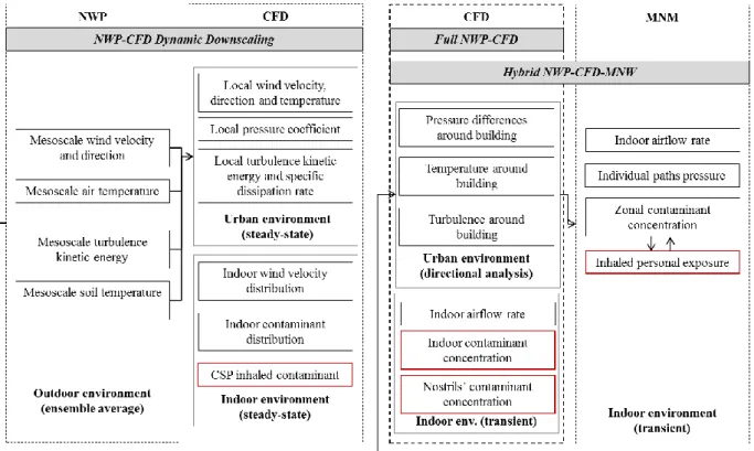
Figure 1-1 shows the flow of the present study.
Figure 1-1. Platform schematic of the present study
~ 5 ~
1.2 INNOVATION TO PREVIOUS RESEARCH
Dynamic downscaling has been historically used to provide regional climate information based on large-scale winds, temperature, water vapor and sea surface temperature from global models1-20~1-22. While most research has focused on eco-resources, recent studies have focused on assessing outdoor air quality through regional downscaling, like urban heat island1-23~1-25.
Several models have overlapped global models analyzed through NWP and microscale models analyzed through CFD using dynamic downscaling techniques. One of these techniques is the use of nested boundary conditions1-26~1-30. Although there are several tactics to overcome the gap between NWP and CFD, there is not yet a straightforward procedure.
From this point of view, the present research presents an innovative quasi-coupling technique to breach the gap between a mesoscale and a microscale environment while at the same time minimizing computational resources and time.
However, none of the previous research has connected mesoscale models to microscale ones for an IAQ analysis that includes the effects of global and urban climate on the human body and the human respiratory system, as the present research proposes.
Furthermore, by applying the present technique of dynamic downscaling and numerical modeling (NWP and CFD), far-reaching analysis can be performed on regions where measured weather data is unavailable as is the case of this study. In this regard, a comprehensive IAQ and inhalation exposure risk analysis method has been developed under minimum requirements of available weather data and computational resources. In this way, a sustainable cost-effective method for IAQ prediction has been proposed.
~ 6 ~
1.3 OBJECTIVES
The main objective of this research is to develop an integrated multi-scale environmental method to analyze inhalation exposure risk from the global climate scale to the human body and respiratory system scale. Realistic continuous flow and pollutant transport from the macro to the micro scale have been analyzed by NWP–CFD–MNM numerical modeling. The following specific objectives can also be derived:
( i ) Prediction of urban air flow field around a target building through NWP–CFD numerical modeling for areas with limited field measurement data,
( ii ) Integration of NWP and CFD to analyze wind pressure coefficient distributions along outside wall surfaces of a building in order to connect the city urban-built environment to the indoor scale in the case of cross-ventilation,
( iii ) Prediction of inhalation exposure risk of a worker in a factory at four different times of the day by using a computer simulated person (CSP) and respiratory system model for short-term exposure (steady-state),
( iv ) Use of MNM to supply average features of flow field and pollutant transport at building and below-building scale between interconnected zones and the outdoor environment to diminish computational load in long-term exposure,
( v ) Application of a full NWP–CFD transient approach based on time-dependent fluctuations of wind pressure coefficient for an accurate transport of city urban-built air flow to the indoor environment for a long-term exposure prediction.
~ 7 ~
References
1-1) Health Effects Institute, WHO. “State of Global Air 2018.” Special Report. Boston, MA: Health Effects Institute, 2018.
1-2) IARC (International Agency for Research on Cancer). “Air Pollution and Cancer.”
IARC Scientific Publication No. 161. Lyon, France: World Health Organization, 2013.
1-3) Shaddick, G, Thomas ML, Green A, Brauer M, Donkelaar A, Burnett R, Chang HH, Cohen A, Dingenen RV, Dora C, Gumy S, Liu Y, Martin R, Waller LA, West J, Zidek JV, and Prüss-Ustün, A. “Data integration model for air quality: a hierarchical approach to the global estimation of exposures to ambient air pollution.” J. R. Stat.
Soc. C, vol. 67, pp. 231–253, 2018.
1-4) U.S. EPA (United States Environmental Protection Agency). “Final Report: Integrated Science Assessment (ISA) for Ozone and Related Photochemical Oxidants” Final Report, Feb. 2013. EPA/600/R-10/076.Washington, DC: U.S. Environmental Protection Agency, 2013.
1-5) Daniels ME Jr, Donilon TE, Bollyky TJ. “The Emerging Global Health Crisis: Non- communicable Diseases in Low- and Middle-Income Countries.” Independent Task Force Report No. 72. New York, NY: Council on Foreign Relations, 2014.
1-6) Sundell J. “On the history of indoor air quality and health.” Indoor Air, vol. 14 Suppl 7, no. Suppl 7, pp. 51–58, 2004.
1-7) Steinemann A, Wargocki P, and Rismanchi B. “Ten questions concerning green buildings and indoor air quality.” Build. Environ., vol. 112, pp. 351–358, 2017.
1-8) Pattinson W, Targino AC, Gibson MD, Krecl P, Cipoli Y, and Sá V. “Quantifying variation in occupational air pollution exposure within a small metropolitan region of Brazil.” Atmos. Environ., vol. 182, pp. 138–154, 2018.
1-9) Dao A, and Bernstein DI. “Occupational exposure and asthma.” Ann. Allergy, Asthma Immunol., 2018 (In Press).
~ 8 ~
1-10) LaDou J. “International occupational health,” Int. J. Hyg. Environ. Health, vol. 206, no. 4–5, pp. 303–313, 2003.
1-11) Spiru P, and Simona PL. “A review on interactions between energy performance of the buildings, outdoor air pollution and the indoor air quality.” Energy Procedia, vol.
128, pp. 179–186, 2017.
1-12) Gupta PK, Lawrence WH, Turner JE, and Autian J. “Toxicological aspects of cyclohexanone,” Toxicol. Appl. Pharmacol., vol. 49, no. 3, pp. 525–533, 1979.
1-13) Höllbacher E, Ters T, Rieder-Gradinger C, and Srebotnik E. “Emissions of indoor air pollutants from six user scenarios in a model room.” Atmos. Environ., vol. 150, pp.
389–394, 2017.
1-14) Deng X, Stull R. “A mesoscale analysis method for surface potential temperature in mountainous and coastal terrain.” Mon. Weather Rev. vol. 133, pp. 389–408, 2005.
1-15) US Department of Energy. “Workshop Report: Research Needs for Wind Resource Characterization.” NREL/TP-500–43521, 2008.
1-16) Tham KW. “Indoor air quality and its effects on humans—A review of challenges and developments in the last 30 years.” Energy Build., vol. 130, pp. 637–650, 2016.
1-17) Carpenter SC. “Energy and IAQ impact of CO2-based demand-controlled ventilation.”
ASHRAE Tran, vol. 102 (2), pp. 80–88, 1996.
1-18) Persily AK, Musser A, Emmerich SJ, and Taylor AW. “Simulations of indoor air quality and ventilation impacts of demand controlled ventilation in commercial and institutional buildings.” NISTIR 7042. Gaithersburg: National Institute of Standards and Technology, 2003.
1-19) Ng L, Musser A, Persily A, and Emmerich S. “Indoor air quality analyses of commercial reference buildings.” Build. Environ. vol. 58, pp. 179–187, 2012.
~ 9 ~
1-20) Gustafson WI, and Leung LR. “Regional Downscaling for Air Quality Assessment: A Reasonable Proposition?” Bulletin of the American Meteorological Society, vol. 88, pp.
1215–1227, 2007.
1-21) Dickinson RE, Errico RM, Giorgi F, and Bates GT. “A regional climate model for the western United States”. Climatic Change, vol. 15, pp. 383–422, 1989.
1-22) Giorgi F, and Mearns LO, 1999 “Introduction to special section: Regional climate modeling revisited” Geophys. Res., vol. 104, pp. 6335-6352, 1999.
1-23) Hogrefe C, Lynn B, Civerolo K, Ku JY, Rosenthal J, Rosenzweig C, Goldberg R, Gaffin S, Knowlton K, and Kinney PL. “Simulating changes in regional air pollution over the eastern United States due to changes in global and regional climate and emissions” Geophys. Res., vol. 109, D22301, 2004.
1-24) Steiner AL, Tonse S, Cohen RC, Goldstein AH, and Harley RA. “Influence of future climate and emissions on regional air quality in California” Geophys. Res., vol. 111, D18303, 2006.
1-25) Jiang GF, and Fast JD. “Modeling the effects of VOC and NOX emission sources on ozone formation in Houston during the TexAQS 2000 field campaign”. Atmos.
Environ., vol. 38, pp. 5071-5085, 2004.
1-26) Kinbara K, Iizuka S, Kuroki M, Kondo A. “Merging WRF and LES models for the analysis of a wind environment in an urban area.” In: Proceedings of the Fifth International Symposium on Computational Wind Engineering. Chapel Hill, NC, May 23–27, 2010.
1-27) Lundquist JK, Mirocha JP, Kosovic B. “Nesting large–eddy simulations within mesoscale simulations in WRF for wind energy applications.” In: Proceedings of the Fifth International Symposium on Computational Wind Engineering. Chapel Hill, NC, May 23–27, 2010.
~ 10 ~
1-28) Ito K. “Integrated numerical approach of computational fluid dynamics and epidemiological model for multi-scale transmission analysis in indoor spaces.” Indoor Built Environ., vol. 23, no. 7, pp. 1029–1049, 2014.
1-29) Murga A, Yoo S-J, Ito K. “Multi stage downscaling procedure to analyse the impact of exposure concentration in a factory on a specific worker through computational fluid dynamics modelling.” Indoor Built Environ., vol. 27, no. 4, pp. 486–498, 2018.
1-30) Murga A, Yoo S-J, Ito K. “A multi-scale exposure concentration analysis in a large factory space using a computational fluid dynamics technique”. In: Proceedings of Healthy Buildings America 2015, USA, July 19-22, pp. 543–546, 2015.
[Previously published documents related to this chapter]
[1] Murga A, Yoo S-J, Ito K. “Multi stage downscaling procedure to analyse the impact of exposure concentration in a factory on a specific worker through computational fluid dynamics modelling.” Indoor Built Environ., vol. 27, no. 4, pp. 486–498, 2018.
[2] Murga A, Yoo S-J, Ito K. “A multi-scale exposure concentration analysis in a large factory space using a computational fluid dynamics technique”. In: Proceedings of Healthy Buildings America 2015, USA, July 19-22, pp. 543–546, 2015.
CHAPTER
2
NUMERICAL MODELING METHODS
2.1 FOREWORD
This research aims to develop an accurate multi-scale numerical modeling method that transfers air flow and pollutant from the global climate scale to the human body and respiratory system scale. From this viewpoint, each scale must be analyzed through suitable mathematical models to describe the physical properties of each environment. In this study, the following scales and models have been used:
For the global climate scale analysis, four mesoscale domains have been implemented from NWP1 to NWP4. The equations of motion in the atmosphere have been discretized through numerical weather prediction (NWP), although it has been typically used for real- time forecasting purposes. NWP has been applied as part of the dynamic downscaling technique for mesoscale air flow, turbulence and temperature prediction.
For the city urban-built scale, building-indoor environment, human body and respiratory system scale, domains CFD1 to CFD4 have been implemented and analyzed through computational fluid dynamics (CFD) to model fluid flow movement.
For the below-building scale, multizone network modeling (MNM) has been applied to domains MNM1–MNM4 for prediction of average features of flow field and contaminant transport through well-mixing approximation and conjunction points.
Governing equations of momentum, energy and scalar transport of each mathematical model are hereby described.
~ 12 ~
2.2 SCALES OF MOTION AND DOMAINS
The present study refers to the analysis of mesoscale domains through NWP and microscales through CFD. However, there are several clarifications in regards to the terms used that need to be made to fully understand the scope of the present research.
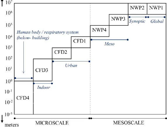
The term “mesoscale” refers to a broad hierarchy of meteorological divisions that correspond to several spatial/temporal scales. As the properties of atmospheric motions vary across scales, the corresponding computational modeling needs to be properly divided to analyze each of these scales2-1~2-3. Figure 2-1 explains the domains and exact spatial scales of atmospheric motion that comprehend the wide term “mesoscale analysis” used in the present study2-4~2-5. Domain NWP1 corresponds to the global-climate scale, domain NWP2 relates to the level of synoptic scale while domains NWP3 and NWP4 conform to a typical mesoscale level.
Figure 2-1. Spatial differentiation of mesoscale and microscale analysis used in this study
~ 13 ~
On the other hand, the term “microscale” used here refers to the smaller scales that have been analyzed below the 104 order (as explained in Figure 2-1). Domains CFD1 and CFD2 conform the urban micro domains, domain CFD3 corresponds to the building level and domain CFD4 analyses the scales below the building level (below-building): the human body and respiratory tract system.
2.3 DISTINCTION BETWEEN NWP AND CFD
Although this study has made the distinction between NWP and CFD, it is important to explain that NWP is a particular form of CFD. NWP specifically studies the motions of the atmosphere as a fluid and therefore uses the equations of fluid dynamics and thermodynamics to predict respective weather results2-6~2-7. The present research makes the distinction between NWP, applied to the mesoscale domains and CFD, applied to the microscale domains, based on the above.
~ 14 ~
2.4 NUMERICAL WEATHER PREDICTION (NWP)
NWP refers to the use of mathematical models of both the atmosphere and oceans to predict weather based on current circumstances. Atmospheric modeling solves the differential equations used to approximate atmospheric flow: continuity equation, conservation of momentum and thermal energy equations. This study uses WRF model version 3.6.1 to analyze domains NWP1 to NWP4.
The weather research and forecasting model (WRF)2-8 is a system developed by multiple agencies that serves atmospheric research and forecasting purposes. Equation solving follows Ooyama’s findings, which use variables that have conservation properties2-9. Following Laprise2-10, equations are formulated using a terrain-following mass vertical coordinate system, further explained in the following sections.
2.4.1 Vertical Coordinate and Variables
η denotes the terrain-following hydrostatic-pressure vertical coordinate explained in equation (2.1):
ph pht
(2.1)
Where phs pht. ph is the pressure hydrostatic component, and phs and pht refer to values along the surface and top boundaries, respectively. This coordinate definition is used in many hydrostatic atmospheric models. η varies from 1 at the surface to 0 at the upper boundary of the domain. This is called a mass vertical coordinate (Figure 2-2).
~ 15 ~
Figure 2-2. Exemplification of the η coordinate
Since ( , )x y is the mass per unit area within the column of the domain at (x, y), the appropriate flux-form variables are:
Vv( , ,U V W), , , (2.2)
Where v( , , )u v w are the covariant velocities in the two horizontal and vertical directions, respectively, is the contravariant vertical velocity and is the potential temperature.
The following non-conserved variables – i.e. not constant – also appear in the governing equations: gz,which represents the geopotential height; p, for pressure; and 1/, which expresses the inverse density.
2.4.2 Governing Equations
Governing equations of motion for atmospheric applications are numerically integrated in this NWP analysis. The governing Euler equations presented in conservative (flux) form, which are the prognostic equations, are described below2-11.
( . ) ( ) ( ) F
tU Vu x pn x px u
(2.3)
( . ) ( ) ( ) F
tV Vv y pn y py v
(2.4)
~ 16 ~
( . ) ( p ) F
tW Vw g n w
(2.5)
( . ) F
t V
(2.6)
( . ) 0
t V
(2.7)
1 (V. ) 0
t gW
(2.8)
The diagnostic relation for the inverse density is:
n
(2.9)
An the equation of state is:
0( d / 0 )
p p R p (2.10)
In the previous equations, x, y and n denote differentiation, .Va x(Ua) y(Va) n( a)
(2.11)
And
. a x x y n
V U a V V a a (2.12)
Where a is a generic variable, Cp /Cv 1.4is the ratio of the heat capacities for dry air, Rd is the gas constant for dry air and p0 is a reference pressure of 105 Pascals. The terms Fu, Fv, Fw and FΘ are the forcing terms arising from model physics, turbulent mixing, spherical projections and earth’s rotation. The prognostic variables are the velocity components zonal and meridional in Cartesian coordinate, vertical velocity w, perturbation potential temperature, perturbation geo-potential, and perturbation surface pressure of dry air.
2.4.3 Model Discretization
In terms of temporal discretization, the model is integrated using a third-order Runge-Kutta time integration scheme (RK3) for a time-split integration2-12. Defining the variables as
( , ,U V W, , ', ',Qm)
with the model equation t R
the solution advances from ( )t to (t t):~ 17 ~
* ( )
3
t t t
R (2.13)
** ( *)
2
t t
R (2.14)
( **)
t t t
tR (2.15)
Where tis the model time step and the superscripts denote time levels.
In terms of spatial discretization, a C grid staggering for the variables is used (Figure 2-3).
In this situation, normal velocities are staggered one-half grid length from the thermodynamic variables and variables indices ( , j, k)i indicate variable locations(x, y, ) (i x,i y,i). Θ is located at mass points and u, v, and w denote u points, v points and w points.
Figure 2-3. Horizontal and vertical grids exemplification
~ 18 ~
2.5 COMPUTATIONAL FLUID DYNAMICS (CFD)
CFD refers to the use of numerical methods and algorithms to solve fluid flow problems that use partial differential equations of mass, momentum and energy by replacing them for a set of algebraic equations solved by a computer. This research uses ANSYS Fluent to provide comprehensive modeling capabilities for incompressible, compressible, laminar and turbulent flows in a steady-state or transient situation by solving the previously mentioned equations2-13.
2.5.1 Basic Equations of Fluid Flow
Fluid motion phenomena are defined by the Navier-Stokes equations expressed in (2.16) and (2.17) for incompressible fluids:
i 0
i
U x
(2.16)
. 1. j
i i i
j i
j i j j i
U U P U U
U v g
t x x x x x
(2.17)
Where Ui represents wind speed (u, v, w components), ρ is the density, v is the kinematic viscosity coefficient, θ is the temperature (or the temperature difference from absolute zero,
0), gi is the gravity component of the acceleration vector in i direction and β is the expansion coefficient.
Equation (2.16) signifies the mass conservation law assuming constant density. Equation (2.17) is the momentum law derived from Newton’s second law and explains the effect of buoyancy. In case of non-isothermal flow field, equation (2.17) can by expressed by the thermal energy transport equation (2.18) with respect to the temperature field.
j
j j j
U S
t x x x
(2.18)
Where α (=λ/Cp·ρ) is the thermal diffusion coefficient and S is the heat generation term (source term).
~ 19 ~
Furthermore, similar to equation (2.18), transport phenomena (e.g. moisture and pollutants) can be defined by the scalar transport equation (2.19):
j '
j j j
U D S
t x x x
(2.19)
Where ϕ is the scalar quantity and D is the diffusion coefficient of the target substance.
Coupled analysis of equations (2.16) and (2.19) make it possible to grasp scalar transport phenomena of incompressible fluids.
2.5.2 Averaging the Equation System
Equations (2.16) to (2.19) are instantaneous physical quantities and include terms expressed in those instantaneous values. Due to the complexity of this equation system, it is impossible to solve them by direct computation. However, an approximation of temporally and spatially consecutive physical quantities into finite ones for an analytical solution can be achieved by discretization. Nonetheless, it is impossible to suppress the fluctuation of the physical quantity below the difference interval. In this situation, it is necessary to apply a method for an approximate solution.
The ensemble average used to achieve this purpose is expressed in equation (2.20):
1
( , ) lim 1 ( , )
N
k i E N i
k
f x t f x t
N
(2.20)
3
' ' '
1
( )i F i i . i i
i
f x G x x f x dx
(2.21)Where subscript E represents ensemble average and subscript F represents spatial averaging. In equation (2.21), the one-dimensional filter function ( )G xi is imposed in three dimensions.
In equations (2.16) to (2.19), instantaneous values are separated into averages and fluctuations. After ensemble average application, the previous equations become:
~ 20 ~
i 0
i
U x
(2.22)
' '
. 1. j
i i i
j i j i
j i j j i j
U U P U U
U v u u g
t x x x x x x
(2.23)
' ' j
j
j j j j
U u
t x x x x
(2.24)
Where Ui, P and θ are average values, ui'and 'are variable and the overbar represents ensemble average values. Equation (2.23) is called the Reynolds equation. Furthermore, the term u ui' 'j in equation (2.23) represents the Reynolds stress and the term u'j' in equation (2.24) is the temperature flux. Originally, the definition of Reynolds stress is approximately the product of density ρ andu ui' 'j ; however, it has been simplified as onlyu ui' 'j .
2.5.3 Model Discretization
The finite volume method (FVM) is one of the most popular discretization methods to represent partial differential equations in their algebraic counterparts2-14~2-15.
FVM denotes the volume that encloses a node point in a mesh. Volume integrals containing divergence are transformed into surface integrals and then calculated as fluxes at the surfaces of each volume, denoted by the following equation:
A A CV
u dA dA S dV
(2.25)Where ρ is the airflow density, ϕ represents the discretization of the velocity components, kinetic energy, dissipation rate and fluid enthalpy. ∇ denotes the scalar gradient and Γ is the diffusion coefficient. In cases of second order accuracy with the Taylor’s expansion approach, the value fcan be explained by the following equation:
,
f SOU r
(2.26)
~ 21 ~
Where and ∇ are the cell-centered value and its gradient and r is the displacement vector from the upstream cell centroid to the face.
2.5.4 Turbulence Models
2.5.4.1 Shear stress transport (SST) k-ω model
In terms of turbulence for the CFD analysis of this study, the RANS Shear Stress Transport (SST) k-ω model – which is based on the standard k-ω model – introduced by Menter has been applied. It has been focused on city urban-built and building-indoor modeling2-16~2-17, as explained in Figure 2-1. This model combines the k-omega and k-epsilon turbulence models, applying the k-omega to the inner region of the boundary layer and the k-epsilon to the free shear flow through blending functions. It also incorporates a damped cross-diffusion derivative term in the omega equation. Furthermore, the turbulent viscosity modeling constants have been modified.
This model is defined by the following equations:
( ) ( i) k k k k
i j j
k ku k G Y S
t x x x
(2.27)
( ) ( i)
i j j
u G Y S
t x x x
(2.28)
Where Gk is the generation of turbulence kinetic energy, Gω is the generation of ω and k and represent the effective diffusivity k and ω. Yk and Yω represent the dissipation of k and ω due to turbulence, Dω is the cross-diffusion term and ρ is density. Sk and Sω are source terms.
Effective diffusivities kand and turbulent viscositytare modelled through equations (2.29), (2.30) and (2.31), respectively:
t k
k
(2.29)
~ 22 ~
t
(2.30)
2 1
1 max 1 ,
*
t
k
F
(2.31)
Where
2 ij ij
(2.32)
1 ,1 1 ,2
1
/ 1 /
k
k k
F F
(2.33)
1 ,1 1 ,2
1
/ 1 /
F F
(2.34)
The previously mentioned blending functions are described below:
41 tanh 1
F (2.35)
1
1 2 2
2
500 4
min max , ,
0.09
k k
y y D y
(2.36)
20 ,2
1 1
max 2 ,10
j j
D k
x x
(2.37)
22 tanh 2
F (2.38)
2 2
max 2 ,500 0.09
k
y y
(2.39)
Where y is distance to surface and D is the positive portion of the cross-diffusion term.
Turbulence production is calculated by the expressions (2.40) and (2.41). S is the stress tensor.
2
k t
G S (2.40)
w k
t
G G
v
(2.41)
Turbulence dissipation of k and ω is represented by equations (2.42) and (2.43):
~ 23 ~
k *
Y k (2.42)
2
Yw (2.43)
The SST model includes the term Dω to blend together the standard k-ω and k-ɛ model, which can be described by equation (2.44):
1 ,2
2(1 ) 1
j j
D F k
x x
(2.44)
Model constants are presented below:
,1 1.176
k ; ,12.0; k,2 1.0; ,21.168; 10.31; i,1 0.075; i,20.0828 2.5.4.2 Low Reynolds k-ɛ model
In general, the standard k-ɛ analyzes turbulence in cases of high Reynolds number;
however, in order to solve turbulence for low Reynold number cases, the low Reynolds number type k-ɛ has been developed2-18. In this study, this model has been applied in the human body and respiratory tract system domain.
This model includes an attenuation function that takes into consideration the wall coordinate y+ and the Reynolds number when obtaining the viscosity coefficient Vt and in the region near the wall surface. A non-slip boundary condition is applied after dividing the wall into sufficient meshes. The model functions f1 and f2 are introduced in the production and dissipation term of turbulence near wall surface.
The following equations embody the low Reynolds k-ɛ model:
' '
. 1. j
i i i
j i j
j i j j i j
U U P U U
U v u u
t x x x x x x
(2.45)
' ' 2
3
i j
i j t ij
j i
U U
u u v k
x x
(2.46)
2 t
v C f k
(2.47)
~ 24 ~
( )
j k k
j
k k
U D P D
t x
(2.48)
1 1 2 2
( )
j k
j
U D C f P C f E
t x k
(2.49)
' ' i
k i j
j
P u u U x
(2.50)
t k
j k j
v k
D v
x x
(2.51)
t
j j
D v v
x x
(2.52)
2
2
k
v k
x (2.53)
Where fμ and f1, f2 represent model functions; D and E have been introduced when is used. In the previous equations fμ= f1= f2=0; D=E=0 and =ɛ.
2.5.5 Radiation Model
This study has considered radiation in the heat transfer simulation. The model introduced, surface-to-surface (S2S), accounts for the radiation exchange in an enclosure of gray-diffuse surfaces. In this model, the energy exchange between two surfaces depends in part of their size, separation distance and orientation.
The main assumption of this model is that any absorption, emission or scattering of radiation can be disregarded, therefore, only “surface-to-surface” radiation need to be considered for analysis. It also accounts for the radiation exchange where gray-diffuse surfaces are located, depending on view factors2-19.
The S2S model uses very low computational resources, making it applicable for building and indoor ventilation analysis2-20.
~ 25 ~
The energy flux that leaves a surface k is composed of directly emitted and reflected energy and can be expressed as:
4
, ,
out k k k k in k
q T q (2.54)
Where qout k, is the energy flux leaving the surface, ɛk is the emissivity (in this case equal to the absorptivity, ), σ is the Stefan-Boltzmann constant, ρk is the density and qin k, is incident flux on surface k from the surroundings.
Incident energy upon a surface can be described by the view factor Fjk, which is the energy leaving surface j and incident on surface k. The incident energy flux qin k, can be expressed as the energy flux leaving surfaces by the following equation:
, ,
1 N
k in k j out j jk
j
A q A q F
(2.55)Where Ak is the area. The view factor reciprocity relationship can be written as:
( 1, 2,3, .)
j jk k kj
A F A F j etc (2.56)
Finally, the equation can be expressed as:
1
J
N
k k k kj j
j
E F J
(2.57)Where Jk is the radiosity (energy given off) and Ek is the emissive power. This equation can be recast into matrix form, with K representing a N M matrix, J is the radiosity vector and E is the emissive power vector, as follows:
KJ E (2.58)
The above is the radiosity matrix equation. Surface cluster temperature can be calculated by area averaging by using equation (2.58):
4 1/ 4
f f
f SC
f
A T
T A
(2.60)~ 26 ~
Where TSC is the temperature and Af and Af are the area and temperature of the face, respectively.
2.5.6 Passive Scalar Transport
In this study, pollutants are assumed to be passive scalars, calculated through the transport equation (2.61) explained below:
Pr
i t
i i i
U v
t x x D x
(2.61)
“Passive scalar” is the assumption that the target substance is the same as air (gas phase).
That is, the Schmit number (Sc=v/D); where v is molecular diffusion coefficient and D is the diffusion coefficient of the target substance in air) is 1. Assuming the Prandtl number as Pr=1 in the transport equation, the diffusion term can be solved through v+vt if flow field analysis is performed and concentration distribution can be analyzed based on flow field.
~ 27 ~
2.6 MULTIZONE NETWORK MODELLING (MNM)
MNM supplies average features of airflow and contaminant transport through interconnected zones in which a building has been divided or in connection with the outdoor environment through pressure differences.
A CFD-only, transient analysis is not practical when analyzing a building with multiple infiltration points because it requires many resources; however, the need for long-term analyses is increasing2-21~2-22. From this point of view, this study proposes a coupling between CFD and MNM that analyzes macroscopic behavior of flow and pollutant transport at a below-building scale2-23. In this study, below-building scale refers to the separate analysis of multiple zones, in which the building has been divided. CONTAM 3.0 has been used for the MNM analysis.
2.6.1 Airflow Analysis
Airflow calculations in CONTAM follow the algorithms developed by AIRNET2-24. The airflow rate from one zone to another Fij is a function of the pressure difference along the flow path Pj – Pi and can be described by the following equation:
( )
ij j i
F f P P (2.62)
The principle of conservation of mass for a transient solution is:
i i i
i i ji i
j
m V
V F F
t t t
(2.63)1
i i i
i t t
i t
m PV
t t RT m
(2.64)
ji 0
j
F
(2.65)Where mi is the mass of air inside a zone and Fi is equal or more than the non-flow processes that could add or remove air from the zone. A non-flow process is a closed system in which mass transfer is not possible.